Mean Value Theorem Math 132 Stewart 3.2 Vanishing derivatives. We - PDF document

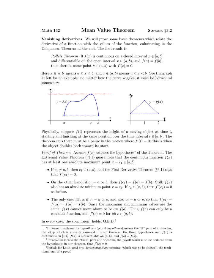
Mean Value Theorem Math 132 Stewart § 3.2 Vanishing derivatives. We will prove some basic theorems which relate the derivative of a function with the values of the function, culminating in the Uniqueness Theorem at the end. The first result is: Rolle’s Theorem: If f ( x ) is continuous on a closed interval x ∈ [ a, b ] and differentiable on the open interval x ∈ ( a, b ), and f ( a ) = f ( b ), then there is some point c ∈ ( a, b ) with f ′ ( c ) = 0. Here x ∈ [ a, b ] means a ≤ x ≤ b , and x ∈ ( a, b ) means a < x < b . See the graph at left for an example: no matter how the curve wiggles, it must be horizontal somewhere. Physically, suppose f ( t ) represents the height of a moving object at time t , starting and finishing at the same position over the time interval t ∈ [ a, b ]. The theorem says there must be a pause in the motion where f ′ ( t ) = 0: this is when the object doubles back toward its start. Proof of Theorem. Assume f ( x ) satisfies the hypotheses ∗ of the Theorem. The Extremal Value Theorem ( § 3.1) guarantees that the continuous function f ( x ) has at least one absolute maximum point x = c 1 ∈ [ a, b ]. • If c 1 � = a, b , then c 1 ∈ ( a, b ), and the First Derivative Theorem ( § 3.1) says that f ′ ( c 1 ) = 0. • On the other hand, if c 1 = a or b , then f ( c 1 ) = f ( a ) = f ( b ). Still, f ( x ) also has an absolute minimum point x = c 2 . If c 2 ∈ ( a, b ), then f ′ ( c 2 ) = 0 as before. • The only case left is if c 1 = a or b , and also c 2 = a or b , so that f ( c 1 ) = f ( c 2 ) = f ( a ) = f ( b ). Since the maximum and minimum values are the same, f ( x ) cannot move above or below f ( a ). Thus, f ( x ) can only be a constant function, and f ′ ( c ) = 0 for all c ∈ ( a, b ). In every case, the conclusion † holds, Q.E.D. ‡ ∗ In formal mathematics, hypothesis (plural hypotheses ) means the “if” part of a theorem, the setup which is given or assumed. In our theorem, the three hypotheses are: f ( x ) is continuous on [ a, b ], f ( x ) is differentiable on ( a, b ), and f ( a ) = f ( b ). † Conclusion means the “then” part of a theorem, the payoff which is to be deduced from the hypothesis: in our theorem, that f ′ ( c ) = 0. ‡ Initials for Latin quod erat demonstrandum meaning “which was to be shown”, the tradi- tional end of a proof.

For Rolle’s Theorem, as for most well-stated theorems, all the hypotheses are necessary to be sure of the conclusion. In the graph at right above, y = g ( x ) has a corner and g ′ (1) does not exist, so just one hypothesis fails at just one point. But already the conclusion is false: g ′ ( c ) = 1 for c < 1 and g ′ ( c ) = − 1 for c > 1, but nowhere is g ′ ( c ) = 0. In physical terms, the velocity jumps instantaneously from 1 to − 1 like an idealized ping-pong ball, and there is no well-defined velocity at the moment of impact. Throughout our theory, the Derivatives versus difference quotients. derivative f ′ ( a ) has been shadowed by the difference quotient, which across an interval [ a, b ] is ∆ ∆ x = f ( b ) − f ( a ) f . Numerically, the difference quotient is an b − a d dx ≈ ∆ f f approximation to the derivative: ∆ x . In physical terms, the difference quotient is the average rate of change of f ( x ) over the interval x ∈ [ a, b ]. Geo- metrically in terms of the graph y = f ( x ), the difference quotient is the slope of the secant line cutting through the points ( a, f ( a )) and ( b, f ( b )). Now we come to the most powerful result of this section, which says that the derivative is sometimes exactly equal to the difference quotient. Mean Value Theorem (MVT): If f ( x ) is continuous on a closed in- terval x ∈ [ a, b ] and differentiable on the open interval x ∈ ( a, b ), then there is some point c ∈ ( a, b ) with f ′ ( c ) = f ( b ) − f ( a ) . b − a See the picture below for an example: as the graph rises from ( a, f ( a )) to ( b, f ( b )), at some points the tangent line must be parallel to the secant line. Note that Rolle’s Theorem is the special case of MVT in which the secant line is horizontal. In fact, we will prove MVT for a general f ( x ) by cooking up a new function g ( x ) for which Rolle’s Theorem applies, then translating Rolle’s conclusion back in terms of f ( x ). Proof of MVT. Suppose f ( x ) satisfies the hypotheses. Then define a new func- tion g ( x ), shown in the picture, which measures the height from the graph y = f ( x ) down to the secant line y = f ( a ) + f ( b ) − f ( a ) ( x − a ): b − a g ( x ) = f ( x ) − f ( a ) − f ( b ) − f ( a ) ( x − a ) . b − a

Then g ( x ) is continuous on [ a, b ] by the Limit Laws ( § 1.6), and differentiable on ( a, b ) by the Derivative Rules ( § 2.3). In fact, g ′ ( x ) = f ′ ( x ) − 0 − f ( b ) − f ( a ) (1 − 0) = f ′ ( x ) − f ( b ) − f ( a ) , b − a b − a since f ( a ) and f ( b ) − f ( a ) are constants (having no x in them). b − a Also, we can easily compute that g ( a ) = g ( b ) = 0, so all the hypotheses of Rolle’s Theorem hold for g ( x ). Thus the conclusion of Rolle’s Theorem also holds: there is some c ∈ ( a, b ) with g ′ ( c ) = 0. That is, g ′ ( c ) = f ′ ( c ) − f ( b ) − f ( a ) = 0 , b − a which means f ′ ( c ) = f ( b ) − f ( a ) , Q.E.D. b − a The Mean Value Theorem does not give any way to find the particular c ∈ ( a, b ) in the conclusion, so if we want this value in a particular case, we must solve for x in the equation f ′ ( x ) = f ( b ) − f ( a ) ; however the Theorem will guarantee b − a that there is some solution. example: Let f ( x ) = 5 √ x − x √ x over the interval [ a, b ] = [0 , 4]. To check the hypotheses of MVT, note that √ x is continuous for all x ≥ 0, and thus over [0 , 4]. As for differentiability: ′ � 5 x 1 / 2 − x 3 / 2 � 2 x − 1 / 2 − 3 f ′ ( x ) = 5 2 x 1 / 2 = is defined for x > 0, and hence over x ∈ (0 , 4): the hypothesis allows f ′ ( a ) = f ′ (0) to be undefined. Thus we conclude there must be some c ∈ (0 , 4) with f ′ ( c ) = f ( b ) − f ( a ) = 2 − 0 4 − 0 = 1 2 . That is, we must solve: b − a 2 x 1 / 2 = 2 x − 1 / 2 − 3 f ′ ( x ) = 5 1 2 , which is equivalent to 3 x + √ x − 5 = 0. Substituting the variable u = √ x gives 3 u 2 + u − 5 = 0, so the Quadratic Formula gives: − 1 ± √ u = √ x = √ 1 2 − 4(3)( − 5) − 1 ± 61 = . 6 2(3) � √ 2 � 61 − 1 The negative solution is impossible, and the positive one gives x = c = ≈ 6 1 . 29, which agrees with the picture.