Machine Learning Lecture 6 Note Compiled by Abhi Ashutosh, Daniel - - PDF document

SLIDE 1

Machine Learning Lecture 6 Note

Compiled by Abhi Ashutosh, Daniel Chen, and Yijun Xiao February 16, 2016

1 Pegasos Algorithm

The Pegasos Algorithm looks very similar to the Perceptron Algorithm. In fact, just by changing a few lines of code in our Perceptron Algorithms, we can get the Pegasos Algorithm. Algorithm 1: Perceptron to Pegasos

1 initialize w1 = 0, t = 0; 2 for iter = 1, 2, ..., 20 do 3

for j = 1, 2, ..., |data| do

4

t = t + 1; ηt =

1 tλ; 5

if yj(wT

t xj) < 1 then 6

wt+1 = (1 − ηtλ)wt + ηtyjxj;

7

else

8

wt+1 = (1 − ηtλ)wt;

9

end

10

end

11

end Side note: We can optimize both the Pegasos and Perceptron Algorithm by using sparse vectors in the case of document classification because most entries in the feature vector x will be zeros. As we discussed in the lecture, the original Pegasos algorithm randomly chooses one data point at each iteration instead of going through each data point in order as shown in Algorithm 1. Pegasos algorithm is an application of the stochastic sub-gradient descent method.

2 Using Pegasos to Solve Other SVM Objec- tives

2.1 Imbalanced data set

Sometimes it may be hard to classify an imbalanced data set where the classi- fication categories are not equally represented. In this case, we want to weigh 1

SLIDE 2

each data point differently by placing more weights on the data points in the underrepresented categories. We can do this very easily by changing our opti- mization problem to min

w w2 2 + CN

2N+

• j:yj=+1

ξj + CN 2N−

• j:yj=−1

ξj where N+, N− are the number of positive data points and negative data points

• respectively. ξj’s are the slack variables.

An intuitive way to think about this is if we want to build a classifier that classifies whether a point is blue or red. If in our data set we only have 1 data point that’s labelled as red and 10 data points labelled as blue, then using the modified objective function is equivalent to duplicating the 1 red point 10 times without explicitly creating more training data.

2.2 Transfer learning

Suppose we want to build a personalized spam classifier for Professor David

• Sontag. However, Professor David only has few of his emails labelled. Professor

Rob, on the other hand, has labelled all of the emails he has ever received as spam or not spam and trained an accurate spam filter on them. Since Professor David and Professor Rob are both Computer Science Professors and run a lab together, we hope that they probably share similar standards for spams/non-

• spams. In this case, a spam classifier built for Professor Rob should work well

to a certain extent for Professor David as well. What should the SVM objective be? (Class ideas: average the weight vectors of both Professors; combine David and Rob’s data and put more weights on David’s data.) One solution is to solve the following modified optimization problem, min

wd,bd

C |Dd|

• x,y∈Dd

max(0, 1 − y(wT

d x + bd)) + 1

2wd − wr2 The idea here is we assume that the weight for Rob is going to be very close to that for David. We then try to penalize the distance between the two. C here can be interpreted as how confident we are that the weights for Rob will be similar to the weights for David. If we are very confident, a low C, then we will really try to minimize the distance between the two weight vectors. If we are not confident, large C, then we are more focused on David’s labelled data.

2.3 Multiclass classification

If we want to extend these ideas further to multi-class classification, we have a number of options. The simplest is called a One-vs-all Classifier in which we learn n classifiers, one for each of the n classes. We could run into issues if we want to classify a point that fell in between our classifiers as we would need to 2

SLIDE 3

decide in which class it belongs. We can predict the most probable class using the formula ˆ y = argmax

k

wT

k x + bk

Another solution is called Multiclass SVM. Here, we put soft restrictions on predicting correct labels for the training data using: w(yj)T xj + b(yj) ≥ w(y′)T xj + b(y′) + 1 − ξj, ∀y′ = yj, ξj ≥ 0, ∀j Notice that we have one slack variable ξj per data point and one set of weights w(k), b(k) for each class k. We could derive a similar Pegasos Algorithm for a multiclass classifier.

3 Kernel Trick

What if the data is not linearly separable? We can create a mapping φ(x) that takes our feature vector x and converts it into a higher dimensional space. Creating a linear classification in this higher dimension and projecting that onto

• ur original feature space will give us a squiggly line classifier.

Kernel tricks allow us to perform the aforementioned classification with little extra cost. For Pegasos algorithm, we can do this by keeping track of just a single variable per data point, αi, and calculating vector w when required. w =

• i

αiyixi Let’s now derive the updating rule for such αi’s. Notice in Algorithm 1, the update rule at each iteration is wt+1 = (1 − ηtλ)wt + ✶[yjwT

t xj < 1] · ηtyjxj

where ✶[condition] is the indicator function. Now instead of xj, yj, let us use x(t), y(t) to denote the data point we randomly selected at iteration t. Substitute ηt, we have wt+1 =

• 1 − 1

t

• wt + 1

λt✶[y(t)wT

t x(t) < 1] · y(t)x(t)

Multiplying both sides with t, rearranging, twt+1 − (t − 1)wt = 1 λ✶[y(t)wT

t x(t) < 1] · y(t)x(t)

As the above equation holds for any t, we have the following t equations          twt+1 − (t − 1)wt = 1

λ✶[y(t)wT t x(t) < 1] · y(t)x(t)

(t − 1)wt − (t − 2)wt−1 = 1

λ✶[y(t−1)wT t−1x(t−1) < 1] · y(t−1)x(t−1)

· · · w2 = 1

λ✶[y(1)wT 1 x(1) < 1] · y(1)x(1)

3

SLIDE 4

Summing over the above t equations and dividing both sides by t, we can have wt+1 = 1 λt

t

• k=1

✶[y(k)wT

k x(k) < 1] · y(k)x(k)

written in the form of summation over i: wt+1 =

• i

  1 λt

t

• k=1

✶[y(k)wT

k x(k) < 1] · ✶[(xi, yi) = (x(k), y(k))]

  yixi All the stuff in the huge parenthesis corresponds to αi we defined earlier. λtα(t+1)

i

counts the number of times data point i appears before iteration t and satisfies yiwT

k xi < 1. This implies a simple updating rule for λtα(t+1) i

: λtα(t+1)

i

= λ(t − 1)α(t)

i

+ ✶[(xi, yi) = (x(t), y(t))] · ✶[yiwT

t xi < 1]

i.e. suppose we draw data point (xi, yi) at iteration t, we increment λtαi by 1 iff yiwT

t xi < 1. The algorithm is shown in Algorithm 2. To simplify the

notations, we denote β(t)

i

= λ(t − 1)α(t)

i .

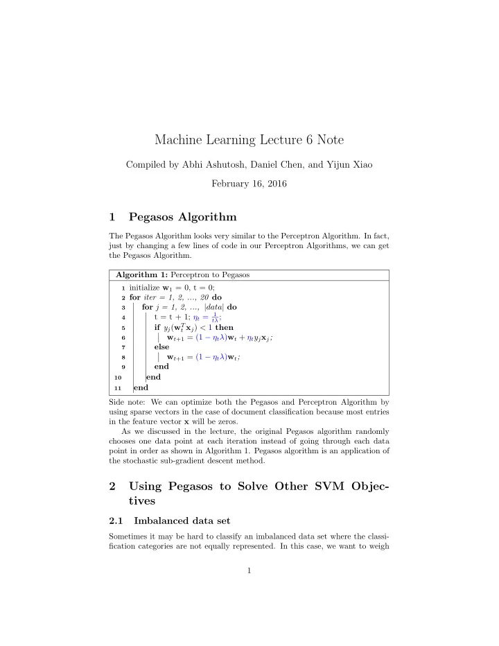
Algorithm 2: Kernelized Pegasos

1 initialize β(1) = 0; 2 for t = 1, 2, ..., T do 3

randomly choose (x(t), y(t)) = (xj, yj) from training data

4

if yj

1 λ(t−1)

• i β(t)

i yixT i xj < 1 then 5

β(t+1)

j

= β(t)

j

+ 1;

6

else

7

β(t+1)

j

= β(t)

j ; 8

end

9

end After convergence, we can get back αi’s using αi =

1 λT β(T +1) i

. In testing time, predictions can be made with ˆ y = sign  

i

αiyixT

i x

  Now suppose we want to use more complex features φ(x) which can be ob- tained by transforming the original features x to a higher dimensional space, all we need to do is to substitute xT

i xj in both training and testing with

φ(xi)T φ(xj). Further notice that φ(x) always appears in the form of dot products. Which indicates we do not necessarily need to explicitly compute it as long as we have 4

SLIDE 5

a formula to calculate the dot products. This is where kernels come into use. Instead of defining the function φ to do the projection, we directly define a kernel function K to calculate the dot product of the projected features. K(xi, xj) = φ(xi)T φ(xj) We can create different kernel functions K(xi, xj) as long as those functions are based on dot products. We can also create new valid kernel functions using

• ther valid kernel functions following certain rules. Examples of popular kernel

functions include Polynomial Kernels, Gaussian Kernels, and many more.

References

Shai Shalev-Shwartz, Yoram Singer, Nathan Srebro, Andrew Cotter. Extended version: Pegasos: Primal Estimated sub-GrAdient SOlver for SVM. Mathemat- ical Programming, Series B, 127(1):3-30, 2011 5