Machine Learning I: Decision Trees AI Class 14 (Ch. 18.118.3) - - PDF document

1

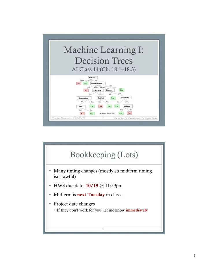
Machine Learning I: Decision Trees

AI Class 14 (Ch. 18.1–18.3)

Cynthia Matuszek – CMSC 671

Material from Dr. Marie desJardin, Dr. Manfred Kerber,

1

Bookkeeping (Lots)

• Many timing changes (mostly so midterm timing

isn’t awful)

• HW3 due date: 10/19 @ 11:59pm
• Midterm is next Tuesday in class
• Project date changes
• If they don’t work for you, let me know immediately

2

2

Today’s Class

• Machine learning
• What is ML?
• Inductive learning
• Supervised
• Unsupervised
• Decision trees
• Later: Bayesian learning, naïve Bayes, and BN

learning ß Review: What is induction?

3

What is Learning?

• “Learning denotes changes in a system that ...

enable a system to do the same task more efficiently the next time.” –Herbert Simon

• “Learning is constructing or modifying

representations of what is being experienced.” –Ryszard Michalski

• “Learning is making useful changes in our minds.”

–Marvin Minsky

4

3

Why Learn?

• Discover previously-unknown new things or structure
• Data mining, scientific discovery
• Fill in skeletal or incomplete domain knowledge
• Large, complex AI systems:
• Cannot be completely derived by hand and
• Require dynamic updating to incorporate new information
• Learning new characteristics expands the domain or expertise and lessens

the “brittleness” of the system

• Build agents that can adapt to users or other agents
• Understand and improve efficiency of human learning
• Use to improve methods for teaching and tutoring people (e.g., better

computer-aided instruction)

5

Pre-Reading Quiz

• What’s supervised learning?
• What’s classification? What’s regression?
• What’s a hypothesis? What’s a hypothesis space?
• What are the training set and test set?
• What is Ockham’s razor?
• What’s unsupervised learning?

6

4

Some Terminology

The Big Idea: given some data, you learn a model of how the world works that lets you predict new data.

• Training Set: Data from which you learn initially.
• Model: What you learn. A “model” of how inputs are

associated with outputs.

• Test set: New data you test tour model against.
• Corpus: A body of data. (pl.: corpora)
• Representation: The computational expression of data

8

Major Paradigms of Machine Learning

• Rote learning: 1:1 mapping from inputs to stored

representation

• You’ve seen a problem before
• Learning by memorization
• Association-based storage and retrieval
• Induction: Specific examples à general

conclusions

• Clustering: Unsupervised grouping of data

9

5

Major Paradigms of Machine Learning

• Analogy: Model is correspondence between two

different representations

• Discovery: Unsupervised, specific goal not given
• Genetic algorithms: “Evolutionary” search

techniques

• Based on an analogy to “survival of the fittest”
• Surprisingly hard to get right/working
• Reinforcement: Feedback (positive or negative

reward) given at the end of a sequence of steps

10

The Classification Problem (1)

• Extrapolate from examples (training

data) to make accurate predictions about future data

• Supervised vs. unsupervised learning
• Learn an unknown function f(X) = Y, where
• X is an input example
• Y is the desired output. (f is the..?)
• Supervised learning implies we are given a training set of (X, Y)

pairs by a “teacher”

• Unsupervised learning means we are only given the Xs and some

(ultimate) feedback function on our performance

11

6

The Classification Problem (2)

• Concept learning or classification

(aka “induction”)

• Given a set of examples of some

concept/class/category:

• Determine if a given example is an

instance of the concept (class member) or not

• If it is, we call it a positive example
• If it is not, it is called a negative example
• Or we can make a probabilistic prediction (e.g., using a

Bayes net)

12

Supervised Concept Learning

• Given a training set of positive and

negative examples of a concept

• Construct a description (model) that

will accurately classify whether future examples are positive or negative

• I.e., learn estimate of function f given a training set:

{(x1, y1), (x2, y2), ..., (xn, yn)} where each yi is either + (positive) or - (negative), or a probability distribution over +/-

13

7

Inductive Learning Framework

• Raw input data from sensors usually

preprocessed to obtain a feature vector, X

• Relevant features for classifying examples
• Each x is a list of (attribute, value) pairs:

X = [Person:Sue, EyeColor:Brown, Age:Young, Sex:Female]

• The number of attributes (a.k.a. features) is fixed (positive, finite)
• Attributes have fixed, finite number # of possible values
• Or continuous within some well-defined space, e.g., “age”
• Examples interpreted as a point in an n-dimensional feature space
• n is the number of attributes

14

Inductive Learning as Search

• Instance space, I, is set of all possible examples
• Defines the language for the training and test instances
• Usually each instance i ∈ I is a feature vector
• Features are also sometimes called attributes or variables
• I: V1 x V2 x … x Vk, i = (v1, v2, …, vk)
• Class variable C gives an instance’s class (to be predicted)
• Model space M defines the possible classifiers
• M: I → C, M = {m1, … mn} (possibly infinite)
• Model space is sometimes defined in terms using same features as the

instance space (not always)

• Training data directs the search for a good (consistent,

complete, simple) hypothesis in the model space

15

8

Model Spaces (1)

• Decision trees
• Partition the instance space into axis-parallel regions
• Labeled with class value
• Nearest-neighbor classifiers
• Partition the instance space into regions defined by centroid

instances (or cluster of k instances)

• Bayesian networks
• Probabilistic dependencies of class on attributes)
• Naïve Bayes: special case of BNs where class à each

attribute

16

Model Spaces (2)

• Neural networks
• Nonlinear feed-forward functions of attribute values
• Support vector machines
• Find a separating plane in a high-dimensional feature

space

• Associative rules (feature values → class)
• First-order logical rules

17

9

Learning Decision Trees

• Goal: Build a decision tree to classify examples as

positive or negative instances of a concept using supervised learning from a training set

• A decision tree is a tree where:
• Each non-leaf node is associated with an attribute (feature)
• Each leaf node has associated with it a classification (+ or -)
• Positive and negative data points
• Each arc is associated with one possible value of the attribute

at the node from which the arc is directed

• Generalization: allow for >2 classes
• e.g., {sell, hold, buy}

19

Learning Decision Trees

• Each non-leaf node is

associated with an attribute (feature)

• Each leaf node is

associated with a classification (+ or -)

• Each arc is associated

with one possible value

• f the attribute at the

node from which the arc is directed

20

10

Will You Buy My Product?

http://www.edureka.co/blog/decision-trees/ 21

Decision Tree-Induced Partition – Example

I

11

Decision Tree-Induced Partition – Example

I

Inductive Learning and Bias

• Suppose that we want to learn a function f(x) = y
• We are given sample (x,y) pairs, as in figure (a)
• Several hypotheses for this function: (b), (c) and (d) (and others)
• A preference for one over others reveals our learning technique’s bias
• Prefer piece-wise functions? (b)
• Prefer a smooth function? (c)
• Prefer a simple function and treat outliers as noise? (d)

25

12

Preference Bias: Ockham’s Razor

• A.k.a. Occam’s Razor, Law of Economy, or Law of Parsimony
• Principle stated by William of Ockham (1285-1347/49), a

scholastic:

• “Non sunt multiplicanda entia praeter necessitatem”
• “Entities are not to be multiplied beyond necessity”
• The simplest consistent explanation is the best
• Smallest decision tree that correctly classifies all training examples
• Finding the provably smallest decision tree is NP-hard!
• So, instead of constructing the absolute smallest tree consistent

with the training examples, construct one that is “pretty small”

26

R&N’s Restaurant Domain

• Model decision a patron makes when deciding

whether to wait for a table

• Two classes (outcomes): wait, leave
• Ten attributes: Alternative available? ∃ Bar? Is it Friday?

Hungry? How full is restaurant? How expensive? Is it raining? Do we have a reservation? What type of restaurant is it? What’s purported waiting time?

• Training set of 12 examples
• ~ 7000 possible cases

27

13

A Training Set

Problem from R&N, table from Dr. Manfred Kerber @ Birmingham, with thanks – www.cs.bham.ac.uk/~mmk/Teaching/AI/l3.html

Outcome Attributes Datum

Decision Tree from Introspection

Problem from R&N, table from Dr. Manfred Kerber @ Birmingham, with thanks – www.cs.bham.ac.uk/~mmk/Teaching/AI/l3.html

14

ID3/C4.5

• A greedy algorithm for decision tree construction
• Ross Quinlan, 1987
• Top-down construction of decision tree by recursively

selecting the “best attribute” to use at current node

• Once attribute is selected for current node, generate children

nodes, one for each possible value of selected attribute

• Partition examples using possible values of this attribute, and

assign these subsets of examples to the appropriate child node

• Repeat for each child node until all examples associated with a

node are either all positive or all negative

30

ID3/C4.5

• 1. Select an attribute for current node
• 2. Generate child nodes
• One for each possible value of selected attribute
• 3. Partition examples (training set) using attribute values
• 4. Assign subsets of examples to appropriate child node
• 5. Repeat for each child node until all examples are either

positive or negative at that node

• These are leaves

31

15

Choosing the Best Attribute

• Key problem: choose which attribute to split a set of examples
• Some possibilities are:
• Random: Select any attribute at random
• Least-Values: Choose the attribute with the smallest number of possible

values

• Most-Values: Choose the attribute with the largest number of possible

values

• Max-Gain: Choose the attribute that has the largest expected information

gain–i.e., the attribute that will result in the smallest expected size of the subtrees rooted at its children

• ID3 uses Max-Gain to select the best attribute

33

Choosing an Attribute

• Idea: a good attribute splits the examples into subsets

that are (ideally) “all positive” or “all negative”

• Which is better: Patrons? or Type?
• Why?

34

16

• What do these approaches split restaurants on,

given the data in the table?

• Random: Patrons or

Wait-time

• Least-values: Patrons
• Most-values: Type
• Max-gain: ???

Restaurant Example

35

French Italian Thai Burger Empty Some Full Y Y Y Y Y Y N N N N N N

Splitting Examples by Testing Attributes

36

examples by #

17

ID3-induced Decision Tree

37

Information Theory 101

• Information is defined as the minimum number of bits

needed to store or send some information

• Wikipedia: “The measure of data, known as information

entropy, is usually expressed by the average number of bits needed for storage or communication”

• Intuitions
• Common words (a, the, dog) are shorter than less common ones

(parliamentarian, foreshadowing)

• In Morse code, common (probable) letters have shorter encodings
• “A Mathematical Theory of Communication,” Bell System

Technical Journal, 1948, Claude E. Shannon, Bell Labs

38

18

Information Theory 103

• Entropy is the average number of bits/message needed to

represent a stream of messages

• Information conveyed by distribution (a.k.a. entropy of P):

I(P) = -(p1*log2 (p1) + p2*log2 (p2) + .. + pn*log2 (pn))

• Examples:
• If P is (0.5, 0.5) then I(P) = 1 à entropy of a fair coin flip
• If P is (0.67, 0.33) then I(P) = 0.92
• If Pis (0.99, 0.01) then I(P) = 0.08
• If P is (1, 0) then I(P) = 0
• As the distribution becomes more skewed, the amount of

information decreases

• ...because I can just predict the most likely element, and usually be right

40

Entropy as Measure of Homogeneity of Examples

• Entropy can be used to characterize the (im)purity of an

arbitrary collection of examples

• Low entropy implies high homogeneity
• Given a collection S (e.g., the table with 12 examples for the

restaurant domain), containing positive and negative examples

• f some target concept, the entropy of S relative to its Boolean

classification is:

I(S) = -(p+*log2 (p+) + p-*log2 (p-))

Entropy([6+, 6-]) = 1 à entropy of the restaurant dataset Entropy([9+, 5-]) = 0.940

41

19

Information Gain

• Information gain is based on:
• Decrease in entropy
• After a dataset is split on an attribute.
• à High homogeneity – e.g., likelihood samples will have

the same class.

• Constructing a decision tree is all about finding

attribute that returns the highest information gain (i.e., the most homogeneous branches)

50

How Well Does it Work?

Decision trees are at least as accurate as human experts!

• A study for diagnosing breast cancer had humans correctly

classifying the examples 65% of the time; the decision tree classified 72% correct

• British Petroleum designed a decision tree for gas-oil separation

for offshore oil platforms that replaced an earlier rule-based expert system

• Cessna designed an airplane flight controller using 90,000

examples and 20 attributes per example

• SKICAT (Sky Image Cataloging and Analysis Tool) used a

decision tree to classify sky objects that were an order of magnitude fainter than was previously possible, with an accuracy

• f over 90%.

53

20

Extensions of the Decision Tree Learning Algorithm

• Using gain ratios
• Real-valued data
• Noisy data and overfitting
• Generation of rules
• Setting parameters
• Cross-validation for experimental validation of performance
• C4.5 is an extension of ID3 that accounts for unavailable

values, continuous attribute value ranges, pruning of decision trees, rule derivation, and so on

54

Real-Valued Data

• Select a set of thresholds defining intervals
• Each interval becomes a discrete value of the attribute
• Use some simple heuristics…
• always divide into quartiles
• Use domain knowledge…
• divide age into infant (0-2), toddler (3 - 5), school-aged (5-8)
• Or treat this as another learning problem
• Try a range of ways to discretize the continuous variable and see

which yield “better results” w.r.t. some metric

• E.g., try midpoint between every pair of values

58

21

Measuring Model Quality

• How good is a model?
• Predictive accuracy
• False positives / false negatives for a given cutoff threshold
• Loss function (accounts for cost of different types of errors)
• Area under the (ROC) curve
• Minimizing loss can lead to problems with overfitting
• Overfitting: coming up with a model that is TOO

specific to your training data

62

Measuring Model Quality

• Training error
• Train on all data; measure error on all data
• Subject to overfitting (of course we’ll make good

predictions on the data on which we trained!)

• Regularization
• Attempt to avoid overfitting
• Explicitly minimize the complexity of the function while

minimizing loss

• Tradeoff is modeled with a regularization parameter

63

22

Cross-Validation

• Holdout cross-validation:
• Divide data into training set and test set
• Train on training set; measure error on test set
• Better than training error, since we are measuring

generalization to new data

• To get a good estimate, we need a reasonably large test set
• But this gives less data to train on, reducing our model

quality!

64

Cross-Validation, cont.

• k-fold cross-validation:
• Divide data into k folds
• Train on k-1 folds, use the kth fold to measure error
• Repeat k times; use average error to measure generalization

accuracy

• Statistically valid and gives good accuracy estimates
• Leave-one-out cross-validation (LOOCV)
• k-fold cross validation where k=N (test data = 1 instance!)
• Quite accurate, but also quite expensive, since it requires

building N models

65

23

Summary: Decision Tree Learning

• Inducing decision trees is one of the most widely used learning

methods in practice

• Can out-perform human experts in many problems
• Strengths include
• Fast
• Simple to implement
• Can convert result to a set of easily interpretable rules
• Empirically valid in many commercial products
• Handles noisy data
• Weaknesses:
• Univariate splits/partitioning using only one attribute at a time so limits

types of possible trees

• Large decision trees may be hard to understand
• Requires fixed-length feature vectors
• Non-incremental (i.e., batch method)

66