Decision tree learning Aim: find a small tree consistent with the - - PowerPoint PPT Presentation

Decision tree learning

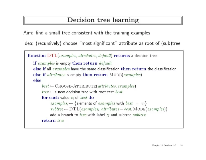
Aim: find a small tree consistent with the training examples Idea: (recursively) choose “most significant” attribute as root of (sub)tree

function DTL(examples, attributes, default) returns a decision tree if examples is empty then return default else if all examples have the same classification then return the classification else if attributes is empty then return Mode(examples) else best ← Choose-Attribute(attributes,examples) tree ← a new decision tree with root test best for each value vi of best do examplesi ← {elements of examples with best = vi} subtree ← DTL(examplesi,attributes − best,Mode(examples)) add a branch to tree with label vi and subtree subtree return tree

Chapter 18, Sections 1–3 24

Choosing an attribute

Idea: a good attribute splits the examples into subsets that are (ideally) “all positive” or “all negative”

None Some Full

Patrons?

French Italian Thai Burger

Type?

Patrons? is a better choice—gives information about the classification

Chapter 18, Sections 1–3 25

Information Theory

♦ Consider communicating two messages (A and B) between two parties ♦ Bits are used to measure message size ♦ If P(A) = 1 and P(B) = 0, how many bits are needed? ♦ If P(A) = .5 and P(B) = .5, how many bits are needed?

Chapter 18, Sections 1–3 26

Information Theory

♦ Consider communicating two messages (A and B) between two parties ♦ Bits are used to measure message size ♦ If P(A) = 1 and P(B) = 0, how many bits are needed? ♦ If P(A) = .5 and P(B) = .5, how many bits are needed? ♦ Information: I(P(v1), ...P(vn)) =

n

i=1 −P(vi) log2 P(vi)

♦ I(1, 0) = 0 bit ♦ I(0.5, 0.5) = −0.5 × log2 0.5 − 0.5 × log2 0.5 = 1 bit

Chapter 18, Sections 1–3 27

Information Theory

♦ Consider communicating two messages (A and B) between two parties ♦ Bits are used to measure message size ♦ If P(A) = 1 and P(B) = 0, how many bits are needed? ♦ If P(A) = .5 and P(B) = .5, how many bits are needed? ♦ Information: I(P(v1), ...P(vn)) =

n

i=1 −P(vi) log2 P(vi)

♦ I(1, 0) = 0 bit ♦ I(0.5, 0.5) = −0.5 × log2 0.5 − 0.5 × log2 0.5 = 1 bit ♦ I measures the information content for communication (or uncertainty in what is already known) ♦ The more one knows, the less to be communicated, the smaller is I ♦ The less one knows, the more to be communicated, the larger is I

Chapter 18, Sections 1–3 28

Using Information Theory

♦ (P(pos), P(neg)): probabilities of positive and negative ♦ Attribute color: black (1,0), white (0,1) ♦ Attribute size: large (.5,.5), small (.5,.5)

Chapter 18, Sections 1–3 29

Using Information Theory

♦ (P(pos), P(neg)): probabilities of positive and negative ♦ Attribute color: black (1,0), white (0,1) ♦ Attribute size: large (.5,.5), small (.5,.5) ♦ Before selecting an attribute

• p = number of positive examples, n = number of negative examples
• Estimating probabilities: P(pos) =

p p+n, P(neg) = n p+n

• Before() = I(P(pos), P(neg))

Chapter 18, Sections 1–3 30

Selecting an Attribute

♦ Evaluating an attribute (e.g., color)

• pi = number of positive examples for value i (e.g., black), ni = number
• f negative ones
• Estimating probabilities for value i: Pi(pos) =

pi pi+ni, Pi(neg) = ni pi+ni

• v values for attribute A (e.g., 2 for color)
• Remainder(A) = After(A) =

v

i=1 pi+ni p+n I(Pi(pos), Pi(neg)) [expected

information]

Chapter 18, Sections 1–3 31

Selecting an Attribute

♦ Evaluating an attribute (e.g., color)

• pi = number of positive examples for value i (e.g., black), ni = number
• f negative ones
• Estimating probabilities for value i: Pi(pos) =

pi pi+ni, Pi(neg) = ni pi+ni

• v values for attribute A (e.g., 2 for color)
• Remainder(A) = After(A) =

v

i=1 pi+ni p+n I(Pi(pos), Pi(neg)) [expected

information] ♦ “Information Gain” (reduction in uncertainty of what is known)

• Gain(A) = Before() − After(A) [Before() has more uncertainty]
• Choose attribute A with the largest Gain(A)

Chapter 18, Sections 1–3 32

Example contd.

Decision tree learned from the 12 examples:

No Yes

Fri/Sat?

None Some Full

Patrons?

No Yes

Hungry? Type?

French Italian Thai Burger

F T T F F T F T

Substantially simpler than “true” tree—a more complex hypothesis isn’t jus- tified by small amount of data

Chapter 18, Sections 1–3 33

Performance measurement

How do we know that h ≈ f? How about measuring the accuracy of h on the examples that were used to learn h?

Chapter 18, Sections 1–3 34

Performance measurement

How do we know that h ≈ f? (Hume’s Problem of Induction)

• 1. Use theorems of computational/statistical learning theory
• 2. Try h on a new test set of examples
• use same distribution over example space as training set
• divide into two disjoint subsets: training and test sets
• prediction accuracy: accuracy on the (unseen) test set

Chapter 18, Sections 1–3 35

Performance measurement

Learning curve = % correct on test set as a function of training set size

0.4 0.5 0.6 0.7 0.8 0.9 1 0 10 20 30 40 50 60 70 80 90100 % correct on test set Training set size

Chapter 18, Sections 1–3 36