Machine Learning I: Decision Trees Schedule mostly finalized Link - - PDF document

1

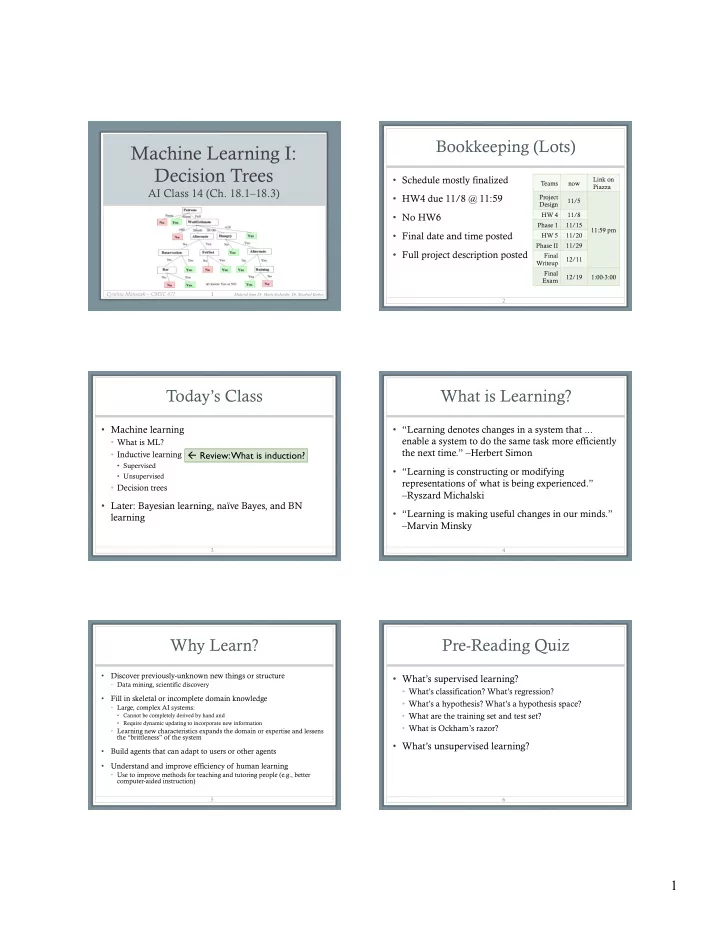
Machine Learning I: Decision Trees

AI Class 14 (Ch. 18.1–18.3)

Cynthia Matuszek – CMSC 671

Material from Dr. Marie desJardin, Dr. Manfred Kerber,

1

Bookkeeping (Lots)

• Schedule mostly finalized
• HW4 due 11/8 @ 11:59
• No HW6
• Final date and time posted
• Full project description posted

2

Teams now Link on Piazza Project Design 11/5 11:59 pm HW 4 11/8 Phase 1 11/15 HW 5 11/20 Phase II 11/29 Final Writeup 12/11 Final Exam 12/19 1:00-3:00

Today’s Class

• Machine learning
• What is ML?
• Inductive learning
• Supervised
• Unsupervised
• Decision trees
• Later: Bayesian learning, naïve Bayes, and BN

learning ß Review: What is induction?

3

What is Learning?

• “Learning denotes changes in a system that ...

enable a system to do the same task more efficiently the next time.” –Herbert Simon

• “Learning is constructing or modifying

representations of what is being experienced.” –Ryszard Michalski

• “Learning is making useful changes in our minds.”

–Marvin Minsky

4

Why Learn?

• Discover previously-unknown new things or structure
• Data mining, scientific discovery
• Fill in skeletal or incomplete domain knowledge
• Large, complex AI systems:
• Cannot be completely derived by hand and
• Require dynamic updating to incorporate new information
• Learning new characteristics expands the domain or expertise and lessens

the “brittleness” of the system

• Build agents that can adapt to users or other agents
• Understand and improve efficiency of human learning
• Use to improve methods for teaching and tutoring people (e.g., better

computer-aided instruction)

5

Pre-Reading Quiz

• What’s supervised learning?
• What’s classification? What’s regression?
• What’s a hypothesis? What’s a hypothesis space?
• What are the training set and test set?
• What is Ockham’s razor?
• What’s unsupervised learning?

6

2

Some Terminology

The Big Idea: given some data, you learn a model of how the world works that lets you predict new data.

• Training Set: Data from which you learn initially.
• Model: What you learn. A “model” of how inputs are

associated with outputs.

• Test set: New data you test tour model against.
• Corpus: A body of data. (pl.: corpora)
• Representation: The computational expression of data

7

A General Model of Learning Agents

8

Major Paradigms of Machine Learning

• Rote learning: 1:1 mapping from inputs to stored

representation

• You’ve seen a problem before
• Learning by memorization
• Association-based storage and retrieval
• Induction: Specific examples à general

conclusions

• Clustering: Unsupervised grouping of data

9

Major Paradigms of Machine Learning

• Analogy: Model is correspondence between two

different representations

• Discovery: Unsupervised, specific goal not given
• Genetic algorithms: “Evolutionary” search

techniques

• Based on an analogy to “survival of the fittest”
• Surprisingly hard to get right/working
• Reinforcement: Feedback (positive or negative

reward) given at the end of a sequence of steps

10

The Classification Problem

• Extrapolate from examples to

make accurate predictions about future data points

• Examples are called training data
• Predict into classes, based
• n attributes (“features”)
• Example: it has tomato sauce,

cheese, and no bread. Is it pizza?

• Example: does this image

contain a cat?

11

yes no

Supervised vs. Unsupervised

• Goal: Learn an unknown function

f (X) = Y, where

• X is an input example
• Y is the desired output. (f is the..?)
• Supervised learning: given a training

set of (X, Y) pairs by a “teacher”

X Y bread cheese tomato sauce pizza ¬ bread ¬ cheese tomato sauce ¬ not pizza bread cheese ¬ tomato sauce gross pizza but still pizza lots more rows…

“class labels” provided

3

Supervised vs. Unsupervised

• Goal: Learn an unknown function

f (X) = Y, where

• X is an input example
• Y is the desired output. (f is the..?)
• Unsupervised learning: only given

Xs and some (eventual) feedback

X bread cheese tomato sauce ¬ bread ¬ cheese tomato sauce bread cheese ¬ tomato sauce lots more rows…

Concept Learning

• Concept learning or classification

(aka “induction”)

• Given a set of examples of some

concept/class/category:

• 1. Determine if a given example is an

instance of the concept (class member) or not

• 2. If it is: positive example
• 3. If it is not: negative example
• 4. Or we can make a probabilistic

prediction (e.g., using a Bayes net)

14

cat?

Supervised Concept Learning

• Given a training set of positive and

negative examples of a concept

• Construct a description (model) that

will accurately classify whether future examples are positive or negative

• I.e., learn estimate of function f given a training set:

{(x1, y1), (x2, y2), ..., (xn, yn)} where each yi is either + (positive) or - (negative), or a probability distribution over +/-

15

Inductive Learning Framework

• Raw input data from sensors preprocessed to obtain

feature vector, X

• Relevant features for classifying examples
• Each X is a list of (attribute, value) pairs
• n attributes (a.k.a. features): fixed, positive, and finite
• Features have fixed, finite number # of possible values
• Or continuous within some well-defined space, e.g., “age”
• Each example is a point in an n-dimensional feature space
• X = [Person:Sue, EyeColor:Brown, Age:Young, Sex:Female]
• X = [Cheese:f, Sauce:t, Bread:t]
• X = [Texture:Fuzzy, Ears:Pointy, Purrs:Yes, Legs:4]

16

Inductive Learning as Search

• Instance space, I, is set of all possible examples
• Defines the language for the training and test instances
• Usually each instance i ∈ I is a feature vector
• Features are also sometimes called attributes or variables

I: V1 × V2 × … × Vk, i = (v1, v2, …, vk)

• Class variable C gives an instance’s class (to be

predicted)

17

Inductive Learning as Search

• C gives an instance’s class
• Model space M defines the possible classifiers
• M: I → C, M = {m1, … mn} (possibly infinite)
• Model space is sometimes defined using same features as

instance space (not always)

• Training data lets us search for a good (consistent,

complete, simple) hypothesis in the model space

• The learned model is a classifier

4

Inductive Learning Pipeline

19

Classifier (trained model) Training data TRAINING

Inductive Learning Pipeline

20

Classifier (trained model) Training data Label: puppy! Test data

Inductive Learning Pipeline

21

Classifier (trained model) Training data Label: puppy! Test data TRAINING

Inductive Learning Pipeline

22

Classifier (trained model) Training data, X Label: + Test data TRAINING

Text- ure Ears Legs Class Fuzzy Round 4

+

Slimy Missing 8

• Fuzzy

Pointy 4

• Fuzzy

Round 4

+

Fuzzy Pointy 4

+

…

x1 = <Fuzzy, Pointy, 4>

Model Spaces (1)

• Decision trees
• Partition the instance space I into axis-parallel regions
• Labeled with class value
• Nearest-neighbor classifiers
• Partition the instance space I into regions defined by centroid

instances (or cluster of k instances)

• Bayesian networks
• Probabilistic dependencies of class on attributes
• Naïve Bayes: special case of BNs where class à each attribute

23

Model Spaces (2)

• Neural networks
• Nonlinear feed-forward functions of attribute values
• Support vector machines
• Find a separating plane in a high-dimensional feature

space

• Associative rules (feature values → class)
• First-order logical rules

24

5

Decision Trees

• Goal: Build a tree to classify examples as positive or

negative instances of a concept using supervised learning from a training set

• A decision tree is a tree where:
• Each non-leaf node is an attribute (feature)
• Each leaf node is a classification (+ or -)
• Positive and negative data points
• Each arc is one possible value of the attribute at the node from

which the arc is directed

• Generalization: allow for >2 classes
• e.g., {sell, hold, buy}

26

Learning Decision Trees

• Each non-leaf node is

associated with an attribute (feature)

• Each leaf node is

associated with a classification (+ or -)

• Each arc is associated

with one possible value

• f the attribute at the

node from which the arc is directed

27

Will You Buy My Product?

http://www.edureka.co/blog/decision-trees/ 28

Decision Tree-Induced Partition – Example

I

Decision Tree-Induced Partition – Example

I

Inductive Learning and Bias

• We want to learn a function f(x) = y
• We are given sample (x,y) pairs, as in figure (a)
• Several hypotheses for this function: (b), (c) and (d) (and others)
• A preference here reveals our learning technique’s bias
• Prefer piece-wise functions? (b)
• Prefer a smooth function? (c)
• Prefer a simple function and treat outliers as noise? (d)

32

6

Preference Bias: Ockham’s Razor

• A.k.a. Occam’s Razor, Law of Economy, or Law of Parsimony
• Stated by William of Ockham (1285-1347/49):
• “Non sunt multiplicanda entia praeter necessitatem”
• “Entities are not to be multiplied beyond necessity”
• “The simplest consistent explanation is the best.”
• Smallest decision tree that correctly classifies all training examples
• Finding the provably smallest decision tree is NP-hard!
• So, instead of constructing the absolute smallest tree consistent

with the training examples, construct one that is “pretty small”

33

R&N’s Restaurant Domain

• Model decision a patron makes when deciding

whether to wait for a table

• Two classes (outcomes): wait, leave
• Ten attributes: Alternative available? ∃ Bar? Is it Friday?

Hungry? How full is restaurant? How expensive? Is it raining? Do we have a reservation? What type of restaurant is it? What’s purported waiting time?

• Training set of 12 examples
• ~ 7000 possible cases

34

A Training Set

Problem from R&N, table from Dr. Manfred Kerber @ Birmingham, with thanks – www.cs.bham.ac.uk/~mmk/Teaching/AI/l3.html

Outcome Attributes Datum

Decision Tree from Introspection

Problem from R&N, table from Dr. Manfred Kerber @ Birmingham, with thanks – www.cs.bham.ac.uk/~mmk/Teaching/AI/l3.html

ID3/C4.5

• A greedy algorithm for decision tree construction
• Ross Quinlan, 1987
• Construct decision tree top-down by recursively

selecting the “best attribute” to use at current node

• 1. Select attribute for current node
• 2. Generate child nodes (one for each possible value of attribute)
• 3. Partition training data using attribute values
• 4. Assign subsets of examples to the appropriate child node
• 5. Repeat for each child node until all examples associated with a

node are either all positive or all negative

37

Bird or Mammal?

1. Select attribute 2. Generate child nodes 3. Partition examples 4. Assign examples to child 5. Repeat until examples are +ve or -ve

Examples (training data) Attributes Outcome Bi- pedal Flies Feath- ers Sparrow Y Y Y B Monkey Y N N M Ostrich Y N Y B Pangolin N N N M Bat Y Y N M Elephant N N N M Chickadee N Y Y B

sparrow, monkey,

• strich,

bat chickadee, pangolin, elephant

Y N Y N

chickadee pangolin, elephant

… Test mouse: <B:N, Fl:N, Fe:N>

7

Choosing the Best Attribute

• Key problem: what attribute to split on?
• Some possibilities are:
• Random: Select any attribute at random
• Least-Values: Choose attribute with smallest number of values
• Most-Values: Choose attribute with largest number of values
• Max-Gain: Choose attribute that has the largest expected

information gain—the attribute that will result in the smallest expected size of the subtrees rooted at its children

• ID3 uses Max-Gain to select the best attribute

39

Choosing an Attribute

• Idea: a good attribute splits the examples into subsets

that are (ideally) “all positive” or “all negative”

• Which is better: Patrons? or Type?
• Why?

40

• What do these approaches split restaurants on,

given the data in the table?

• Random: Patrons or

Type

• Least-values: Patrons
• Most-values: Type
• Max-gain: ???

Restaurant Example

41

French Italian Thai Burger Empty Some Full Y Y Y Y Y N N N N N

Splitting Examples by Testing Attributes

42

examples by #

ID3-induced Decision Tree

43

Information Theory 101

• Information: the minimum number of bits needed

to store or send some information

• Wikipedia: “The measure of data, known as information

entropy, is usually expressed by the average number of bits needed for storage or communication”

• Intuition: minimize effort to communicate/store
• Common words (a, the, dog) are shorter than less

common ones (parliamentarian, foreshadowing)

• In Morse code, common (probable) letters have shorter

encodings

“A Mathematical Theory of Communication,” Bell System Technical Journal, 1948, Claude E. Shannon, Bell Labs

8

Information Theory 102

• Information is measured in bits.
• Information in a message depends on its probability.
• Given n equally probable possible messages, what is

probability pn of each one? 1/n

• Information conveyed by a message is log2(n) = -log2(p)
• Example: with 16 possible messages, log2(16) = 4, and

we need 4 bits to identify/send each message

45

Information Theory 102.b

• Information conveyed by a message is log2(n) = -log2(p)
• Given a probability distribution for n messages:

P = (p1,p2…pn)

• The information conveyed by that distribution is:

I(P) = -(p1*log2(p1) + p2*log2(p2) + .. + pn*log2(pn))

• This is the entropy of P.

46

Information Theory 103

• Entropy: average number of bits (per message) needed to

represent a stream of messages

I(P) = -(p1*log2 (p1) + p2*log2 (p2) + .. + pn*log2 (pn))

• Examples:
• P = (0.5, 0.5) : I(P) = 1

à entropy of a fair coin flip

• P = (0.67, 0.33) : I(P) = 0.92
• P = (0.99, 0.01) : I(P) = 0.08
• P = (1, 0) : I(P) = 0
• As the distribution becomes more skewed, the amount of

information decreases. Why?

• Because I can just predict the most likely element, and usually

be right

47

Entropy as Measure of Homogeneity of Examples

• Entropy can be used to characterize the (im)purity of

an arbitrary collection of examples

• Low entropy implies high homogeneity
• Given a collection S (like the table of 12 examples for the

restaurant domain), containing positive and negative examples

• f some target concept, the entropy of S relative to its Boolean

classification is:

I(S) = -(p+*log2 (p+) + p-*log2 (p-))

Entropy([6+, 6-]) = 1 à entropy of the restaurant dataset Entropy([9+, 5-]) = 0.940

48

Information Gain

• Information gain: how much entropy decreases

(homogeneity increases) when a dataset is split on an attribute.

• High homogeneity à high likelihood samples will have the

same class

• Constructing a decision tree is all about finding

attribute that returns the highest information gain (i.e., the most homogeneous branches)

54

Information Gain, cont.

• Use to rank attributes and build DT (decision tree)!
• Choose nodes using attribute with greatest gain
• à means least information remaining after split
• I.e., subsets are all as skewed as possible
• Why?
• Create small decision trees: predictions can be made with

few attribute tests

• Try to find a minimal process that still captures the data

(Occam’s Razor)

55

9

How Well Does it Work?

At least as accurate as human experts (sometimes)

• Diagnosing breast cancer: humans correct 65% of the time;

decision tree classified 72% correct

• BP designed a decision tree for gas-oil separation for offshore
• il platforms; replaced an earlier rule-based expert system
• Cessna designed an airplane flight controller using 90,000

examples and 20 attributes per example

• SKICAT (Sky Image Cataloging and Analysis Tool) used a

DT to classify sky objects an order of magnitude fainter than was previously possible, with an accuracy of over 90%.

60

Extensions of the Decision Tree Learning Algorithm

• Using gain ratios
• Real-valued data
• Noisy data and overfitting
• Generation of rules
• Setting parameters
• Cross-validation for experimental validation of performance

C4.5 is a (more applicable) extension of ID3 that accounts for real-world problems: unavailable values, continuous attributes, pruning decision trees, rule derivation, …

61

Real-Valued Data

• Select a set of thresholds defining intervals
• Each interval becomes a discrete value of the attribute
• Use some simple heuristics…
• always divide into quartiles
• Use domain knowledge…
• divide age into infant (0-2), toddler (3 - 5), school-aged (5-8)
• Or treat this as another learning problem
• Try a range of ways to discretize the continuous variable and see

which yield “better results” w.r.t. some metric

• E.g., try midpoint between every pair of values

65

Converting Decision Trees to Rules

• 1 rule for each path in tree (from root to a leaf)
• Left-hand side: labels
• f nodes and arcs

Pa.=None à Don’t wait Pa.=Some à Wait Pa.=F ∧ Hu.=No à Don’t wait etc…

• Resulting rules can be simplified and reasoned over

67

Simplifying Rules

• Let LHS be the left hand side of a rule
• Let LHS' be obtained from LHS by eliminating

some conditions

• We can certainly replace LHS by LHS' in this rule if

the subsets of the training set that satisfy respectively LHS and LHS' are equal

• A rule may be eliminated by using metaconditions

such as “if no other rule applies”

68

Noisy Data

• Many kinds of “noise” can occur in the examples:
• Two examples have same attribute/value pairs, but

different classifications

• Some values of attributes are incorrect because of errors in

data acquisition or preprocessing phase

• The classification is wrong (e.g., + instead of -) because of

some error

• Attributes irrelevant to the decision-making process
• Color of a die is irrelevant to its outcome
• Can still be in training data, can be chosen as an attribute

69

10

Overfitting

70

• Sometimes, model fits training data well but doesn’t

do well on test data

• Can be it “overfit” to

the training data

• Model is too specific

to training data

• Doesn’t generalize to

new information well

• Learned model: (Y∧Y∧YàB ∨ Y∧N∧NàM ∨ ...)

Examples (training data) Attributes Outcome Bi-pedal Flies Feath-ers Sparrow Y Y Y B Monkey Y N N M Ostrich Y N Y B Bat Y Y N M Elephant N N N M

Noisy Data and Overfitting

• Irrelevant attributes à
• verfitting
• If hypothesis space has many

dimensions (many attributes), may find meaningless regularity

• Ex: Name starts with [A-M] à Mammal
• One fix: prune lower nodes in the decision tree
• Ex: if Gain of best attribute at a node is below a threshold,

stop; make a leaf rather than generating children

71 Examples (training data) Attributes Class Bi- pedal Feath- ers Sparrow Y Y B Monkey Y N M Ostrich Y Y B Bat Y N M Elephant N N M

Measuring Model Quality

• How good is a model?
• Predictive accuracy on test data
• False positives / false negatives for a given cutoff threshold
• Loss function (accounts for cost of different types of errors)
• Area under the (ROC) curve
• Minimizing loss can lead to problems with overfitting
• Overfitting: coming up with a model that is TOO

specific to your training data

72

Measuring Model Quality

• Training error
• Train on all data; measure error on all data
• Subject to overfitting (of course we’ll make good

predictions on the data on which we trained!)

• Regularization
• Attempt to avoid overfitting
• Explicitly minimize the complexity of the function while

minimizing loss

• Tradeoff is modeled with a regularization parameter

73

Cross-Validation

• Holdout cross-validation:
• Divide data into training set and test set
• Train on training set; measure error on test set
• Better than training error, since we are measuring

generalization to new data

• To get a good estimate, we need a reasonably large test set
• But this gives less data to train on, reducing our model

quality!

74

Cross-Validation, cont.

• k-fold cross-validation:
• Divide data into k folds
• Train on k-1 folds, use the kth fold to measure error
• Repeat k times; use average error to measure generalization

accuracy

• Statistically valid and gives good accuracy estimates
• Leave-one-out cross-validation (LOOCV)
• k-fold cross validation where k=N (test data = 1 instance!)
• Quite accurate, but also quite expensive, since it requires

building N models

75

11

Summary: Decision Tree Learning

• One of the most widely used learning methods in practice
• Can out-perform human experts in many problems
• Strengths include
• Fast
• Simple to implement
• Can convert result to a set of easily interpretable rules
• Empirically valid in many commercial products
• Handles noisy data
• Weaknesses:
• Univariate splits/partitioning using only one attribute at a time

(limits types of possible trees)

• Large decision trees may be hard to understand
• Requires fixed-length feature vectors
• Non-incremental (i.e., batch method)

76