Machine Learning for Computational Linguistics May 24, 2016 . - - PDF document

SLIDE 1

Machine Learning for Computational Linguistics

Unsupervised learning Çağrı Çöltekin

University of Tübingen Seminar für Sprachwissenschaft

May 24, 2016

Practical matters Summary Introduction Clustering K-means Mixture densities Hierarchical clustering PCA

Homework 1

Common confusions (mainly about bigrams):

▶ Word ngrams (typically) do not cross sentence boundaries ▶ Order is important in a bigram ▶ While calculating conditional probabilities and PMI for

bigrams, you need to use probability of a word given it is the fjrst/second word in the bigram, not its unigram probability

▶ The base of logarithm does not matter for information

theoretic measures. Base only changes the ‘unit’. As long as you are consistent, using any base is fjne.

Ç. Çöltekin, SfS / University of Tübingen May 24, 2016 1 / 40 Practical matters Summary Introduction Clustering K-means Mixture densities Hierarchical clustering PCA

Projects

▶ Please send me short project proposal document (about one

page) by June 13 with

▶ the list of the project members ▶ a title, brief description ▶ whether you have already obtained data for the project or not ▶ the methods you intend to apply

▶ and let me know as soon as you formed your project team

Ç. Çöltekin, SfS / University of Tübingen May 24, 2016 2 / 40 Practical matters Summary Introduction Clustering K-means Mixture densities Hierarchical clustering PCA

Supervised learning

▶ The methods we studied so far are instances of supervised

learning

▶ In supervised learning, we have a set of predictors x, and want

to predict a response or outcome variable y

▶ During training we have access to both input and output

variables

▶ Typically, training consist of estimating parameters w of a

model

▶ During prediction, we are given x and make predictions based

• n what we learned (e.g., parameter estimates) during training

Ç. Çöltekin, SfS / University of Tübingen May 24, 2016 3 / 40 Practical matters Summary Introduction Clustering K-means Mixture densities Hierarchical clustering PCA

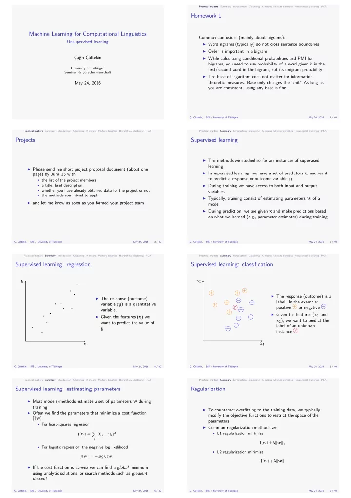
Supervised learning: regression

x y

▶ The response (outcome)

variable (y) is a quantitative variable.

▶ Given the features (x) we

want to predict the value of y

Ç. Çöltekin, SfS / University of Tübingen May 24, 2016 4 / 40 Practical matters Summary Introduction Clustering K-means Mixture densities Hierarchical clustering PCA

Supervised learning: classifjcation

x1 x2 + + + + + + − − − − − − − ?

▶ The response (outcome) is a

• label. In the example:

positive + or negative −

▶ Given the features (x1 and

x2), we want to predict the label of an unknown instance ?

Ç. Çöltekin, SfS / University of Tübingen May 24, 2016 5 / 40 Practical matters Summary Introduction Clustering K-means Mixture densities Hierarchical clustering PCA

Supervised learning: estimating parameters

▶ Most models/methods estimate a set of parameters w during

training

▶ Often we fjnd the parameters that minimize a cost function

J(w)

▶ For least-squares regression

J(w) = ∑

i

(ˆ yi − yi)2

▶ For logistic regression, the negative log likelihood

J(w) = −logL(w)

▶ If the cost function is convex we can fjnd a global minimum

using analytic solutions, or search methods such as gradient descent

Ç. Çöltekin, SfS / University of Tübingen May 24, 2016 6 / 40 Practical matters Summary Introduction Clustering K-means Mixture densities Hierarchical clustering PCA

Regularization

▶ To counteract overfjtting to the training data, we typically

modify the objective functions to restrict the space of the parameters

▶ Common regularization methods are

▶ L1 regularization minimize

J(w) + λ∥w∥1

▶ L2 regularization minimize

J(w) + λ∥w∥

Ç. Çöltekin, SfS / University of Tübingen May 24, 2016 7 / 40

SLIDE 2

Practical matters Summary Introduction Clustering K-means Mixture densities Hierarchical clustering PCA

Unsupervised learning

▶ In unsupervised learning, we do not have labels ▶ Our aim is to fjnd useful patterns/structure in the data ▶ Typical unsupervised methods include

▶ Clustering: fjnd related groups of instances ▶ Density estimation: fjnd a probability distribution that explains

the data

▶ Dimensionality reduction: fjnd a accurate/useful lower

dimensional representation of the data

▶ Evaluation is diffjcult: we do not have ‘true’ labels/values ▶ Sometimes unsupervised methods can be used in conjunction

with the supervised methods

Ç. Çöltekin, SfS / University of Tübingen May 24, 2016 8 / 40 Practical matters Summary Introduction Clustering K-means Mixture densities Hierarchical clustering PCA

Clustering

▶ Our aim is to fjnd groups of instances/items that are similar

to each other

▶ Clustering similar languages, dialects, documents,

users/authors …

▶ The distance measure is important (but also application

specifjc)

▶ Clustering can be hierarchical or non-hierarchical ▶ Clustering can be bottom-up (agglomerative) or top-down

(divisive)

▶ For most (useful) problems we cannot fjnd globally optimum

solutions, we often rely on greedy algorithms fjnding local

• ptima.

Ç. Çöltekin, SfS / University of Tübingen May 24, 2016 9 / 40 Practical matters Summary Introduction Clustering K-means Mixture densities Hierarchical clustering PCA

Clustering example in two dimensions

x1 x2

▶ Unlike classifjcation we do

not have labels

▶ We want to fjnd ‘natural’

groups in the data

▶ Intuitively, similar or closer

data points are grouped together

Ç. Çöltekin, SfS / University of Tübingen May 24, 2016 10 / 40 Practical matters Summary Introduction Clustering K-means Mixture densities Hierarchical clustering PCA

Similarity and distance

▶ The notion of distance (similarity) is very important in

• clustering. A distance measure D,

▶ is symmetric: D(a, b) = D(b, a) ▶ non-negative: D(a, b) ⩾ 0 for all a, b, and it D(a, b) = 0 ifg

a = b

▶ obeys triangle inequality: D(a, b) + D(b, c) ⩾ D(a, c)

▶ The choice of distance is application specifjc ▶ A few common choices:

▶ Euclidean distance: ∥a − b∥ =

√∑k

j=1(aj − bj)2

▶ Manhattan distance: ∥a − b∥1 = ∑k

j=1|aj − bj|

▶ We will often face with defjning distance measures between

linguistic units (letters, words, sentences, documents, …)

Ç. Çöltekin, SfS / University of Tübingen May 24, 2016 11 / 40 Practical matters Summary Introduction Clustering K-means Mixture densities Hierarchical clustering PCA

How to do clustering

Most clustering algorithms try to minimize the scatter within each

• cluster. Which is equivalent to maximizing the scatter between

clusters x1 x2 1 2

K

∑

k=1

∑

C(a)=k

∑

C(b)=k

d(a, b)

▶

1 2

K

∑

k=1

∑

C(a)=k

∑

C(b)̸=k

d(a, b) Exact solution (fjnding global optimum) is not possible for realistic

• data. We use methods that fjnd a local minimum.

Ç. Çöltekin, SfS / University of Tübingen May 24, 2016 12 / 40 Practical matters Summary Introduction Clustering K-means Mixture densities Hierarchical clustering PCA

K-means clustering

K-means is a popular method for clustering.

• 1. Randomly choose centroids, m1, . . . , mK, representing K

clusters

• 2. Repeat until convergence

▶ Assign each data point to the cluster of the nearest centroid ▶ Re-calculate the centroid locations based on the assignments

Efgectively, we are fjnding a local minimum of the sum of squared Euclidean distance within each cluster 1 2

K

∑

k=1

∑

C(a)=k

∑

C(b)=k

∥a − b∥2

Ç. Çöltekin, SfS / University of Tübingen May 24, 2016 13 / 40 Practical matters Summary Introduction Clustering K-means Mixture densities Hierarchical clustering PCA

K-means clustering: visualization

1 2 3 4 5 1 2 3 4 5

▶ The data ▶ Set cluster centroids

randomly

▶ Assign data points to

closest centroid

▶ Recalculate the

centroids

Ç. Çöltekin, SfS / University of Tübingen May 24, 2016 14 / 40 Practical matters Summary Introduction Clustering K-means Mixture densities Hierarchical clustering PCA

K-means clustering: visualization

1 2 3 4 5 1 2 3 4 5

▶ The data ▶ Set cluster centroids

randomly

▶ Assign data points to

closest centroid

▶ Recalculate the

centroids

Ç. Çöltekin, SfS / University of Tübingen May 24, 2016 14 / 40

SLIDE 3

Practical matters Summary Introduction Clustering K-means Mixture densities Hierarchical clustering PCA

K-means clustering: visualization

1 2 3 4 5 1 2 3 4 5

▶ The data ▶ Set cluster centroids

randomly

▶ Assign data points to

closest centroid

▶ Recalculate the

centroids

Ç. Çöltekin, SfS / University of Tübingen May 24, 2016 14 / 40 Practical matters Summary Introduction Clustering K-means Mixture densities Hierarchical clustering PCA

K-means clustering: visualization

1 2 3 4 5 1 2 3 4 5

▶ The data ▶ Set cluster centroids

randomly

▶ Assign data points to

closest centroid

▶ Recalculate the

centroids

Ç. Çöltekin, SfS / University of Tübingen May 24, 2016 14 / 40 Practical matters Summary Introduction Clustering K-means Mixture densities Hierarchical clustering PCA

K-means clustering: visualization

1 2 3 4 5 1 2 3 4 5

▶ The data ▶ Set cluster centroids

randomly

▶ Assign data points to

closest centroid

▶ Recalculate the

centroids

Ç. Çöltekin, SfS / University of Tübingen May 24, 2016 14 / 40 Practical matters Summary Introduction Clustering K-means Mixture densities Hierarchical clustering PCA

K-means clustering: visualization

1 2 3 4 5 1 2 3 4 5

▶ The data ▶ Set cluster centroids

randomly

▶ Assign data points to

closest centroid

▶ Recalculate the

centroids

Ç. Çöltekin, SfS / University of Tübingen May 24, 2016 14 / 40 Practical matters Summary Introduction Clustering K-means Mixture densities Hierarchical clustering PCA

K-means clustering: visualization

1 2 3 4 5 1 2 3 4 5

▶ The data ▶ Set cluster centroids

randomly

▶ Assign data points to

closest centroid

▶ Recalculate the

centroids

Ç. Çöltekin, SfS / University of Tübingen May 24, 2016 14 / 40 Practical matters Summary Introduction Clustering K-means Mixture densities Hierarchical clustering PCA

K-means clustering: visualization

1 2 3 4 5 1 2 3 4 5

▶ The data ▶ Set cluster centroids

randomly

▶ Assign data points to

closest centroid

▶ Recalculate the

centroids

Ç. Çöltekin, SfS / University of Tübingen May 24, 2016 14 / 40 Practical matters Summary Introduction Clustering K-means Mixture densities Hierarchical clustering PCA

K-means: issues

▶ K-means requires the data points to be on an Euclidean space ▶ K-means is sensitive to outliers ▶ The results are highly sensitive to initialization

▶ There are some smarter ways to select initial points ▶ One can do multiple initializations, and pick the best (with

lowest within-group squares)

▶ It works well with approximately equal sized round shaped

clusters

▶ We need to specify number of clusters in advance

Ç. Çöltekin, SfS / University of Tübingen May 24, 2016 15 / 40 Practical matters Summary Introduction Clustering K-means Mixture densities Hierarchical clustering PCA

How many clusters?

▶ The number of clusters is defjned for some problems, e.g.,

classifying news into a fjxed set of topics/interests

▶ For others, there is no clear way to select the best number of

clusters

▶ The error (within cluster scatter) always decreases with

increasing number of clusters, using a test set or cross validation is not useful either

▶ A common approach is clustering for multiple K values, and

picking where there is an ‘elbow’ in the graph against the error function

Ç. Çöltekin, SfS / University of Tübingen May 24, 2016 16 / 40

SLIDE 4

Practical matters Summary Introduction Clustering K-means Mixture densities Hierarchical clustering PCA

How many clusters?

K J(w)

1 2 3 4 5 6 7 8 9 40 80 120 160

Ç. Çöltekin, SfS / University of Tübingen May 24, 2016 17 / 40 Practical matters Summary Introduction Clustering K-means Mixture densities Hierarchical clustering PCA

K-medoids

▶ K-means requires the data to be on an Euclidean space ▶ Sometimes, we only have distances between the data points,

the features do not lie in an Euclidean space

▶ K-medoids algorithm is an alternation of K-means ▶ Instead of calculating centroids, we try to fjnd most typical

data point at each iteration

▶ It is less sensitive to outliers ▶ It is computationally more expensive than K-means

Ç. Çöltekin, SfS / University of Tübingen May 24, 2016 18 / 40 Practical matters Summary Introduction Clustering K-means Mixture densities Hierarchical clustering PCA

Density estimation

▶ K-means treats all data points in a cluster equally ▶ A ‘soft’ version of K-means is density estimation for Gaussian

mixtures, where

▶ We assume the data comes from a mixture of K Gaussian

distributions

▶ We try to fjnd the parameters of each distribution that

maximizes the probability of the data

▶ Unlike K-means, mixture of Gaussians assigns probabilities for

each data point belonging to one of the clusters

▶ It is typically estimated using the expectation-maximization

(EM) algorithm

Ç. Çöltekin, SfS / University of Tübingen May 24, 2016 19 / 40 Practical matters Summary Introduction Clustering K-means Mixture densities Hierarchical clustering PCA

Density estimation using the EM algorithm

▶ The EM algorithm (or its variations) is used in many

(unsupervised) learning models with latent/hidden variables

▶ It is closely related to the K-means algorithm

• 1. Randomly initialize the parameters of K Gaussian distributions

(µ, Σ)

• 2. Iterate until convergence:

E-step Compute probability of each data point belonging to each cluster, given the parameters M-step Re-estimate the mixture density parameters using the probabilities estimated in the E-step

Ç. Çöltekin, SfS / University of Tübingen May 24, 2016 20 / 40 Practical matters Summary Introduction Clustering K-means Mixture densities Hierarchical clustering PCA

Hierarchical clustering

▶ Instead of fmat division to clusters as in K-means, hierarchical

clustering builds a hierarchy based on similarity of the data points

▶ There are two main ‘modes of operation’:

Bottom-up or agglomerative clustering starts with individual data points, and merges until a single root node is reached Top-down or divisive clustering starts with a single cluster, and splits until all leaves are single data points

▶ Hierarchical clustering operates on difgerences ▶ The result is a binary tree called dendrogram ▶ Dendrogram are easy to interpret (especially if data is

hierarchical)

▶ The algorithm does not commit to the number of clusters K

from the start, dendrogram could be ‘cut’ at any height for a particular number of clusters

Ç. Çöltekin, SfS / University of Tübingen May 24, 2016 21 / 40 Practical matters Summary Introduction Clustering K-means Mixture densities Hierarchical clustering PCA

Agglomerative clustering

• 1. Compute the

similarity/distance matrix

• 2. Assign each data point to its
• wn cluster
• 3. Repeat until no cluster left

to merge

▶ Pick two clusters that are

most similar to each other

▶ Merge them into a single

cluster

1 2 3 4 5

Ç. Çöltekin, SfS / University of Tübingen May 24, 2016 22 / 40 Practical matters Summary Introduction Clustering K-means Mixture densities Hierarchical clustering PCA

Agglomerative clustering demonstration

1 2 3 4 5 x1 x2 1 2 3 4 5

Ç. Çöltekin, SfS / University of Tübingen May 24, 2016 23 / 40 Practical matters Summary Introduction Clustering K-means Mixture densities Hierarchical clustering PCA

How to calculate between cluster distances

Complete maximal inter-cluster distance Single minimal inter-cluster distance Average mean inter-cluster distance Centroid distance between the centroids x1 x2 1 2 3 4 5 Note: single linkage tends to produce unbalanced trees.

Ç. Çöltekin, SfS / University of Tübingen May 24, 2016 24 / 40

SLIDE 5

Practical matters Summary Introduction Clustering K-means Mixture densities Hierarchical clustering PCA

How to calculate between cluster distances

Complete maximal inter-cluster distance Single minimal inter-cluster distance Average mean inter-cluster distance Centroid distance between the centroids x1 x2 1 2 3 4 5 Note: single linkage tends to produce unbalanced trees.

Ç. Çöltekin, SfS / University of Tübingen May 24, 2016 24 / 40 Practical matters Summary Introduction Clustering K-means Mixture densities Hierarchical clustering PCA

How to calculate between cluster distances

Complete maximal inter-cluster distance Single minimal inter-cluster distance Average mean inter-cluster distance Centroid distance between the centroids x1 x2 1 2 3 4 5 Note: single linkage tends to produce unbalanced trees.

Ç. Çöltekin, SfS / University of Tübingen May 24, 2016 24 / 40 Practical matters Summary Introduction Clustering K-means Mixture densities Hierarchical clustering PCA

How to calculate between cluster distances

Complete maximal inter-cluster distance Single minimal inter-cluster distance Average mean inter-cluster distance Centroid distance between the centroids x1 x2 1 2 3 4 5 Note: single linkage tends to produce unbalanced trees.

Ç. Çöltekin, SfS / University of Tübingen May 24, 2016 24 / 40 Practical matters Summary Introduction Clustering K-means Mixture densities Hierarchical clustering PCA

Clustering: some closing notes

▶ We do not have proper evaluation procedures for clustering

results (for unsupervised learning in general)

▶ Clustering is typically unstable, slight changes in the data or

parameter choices may change the results drastically

▶ Approaches against instability include some validation

methods, or producing ‘probabilistic’ dendrograms by running clustering with difgerent options

Ç. Çöltekin, SfS / University of Tübingen May 24, 2016 25 / 40 Practical matters Summary Introduction Clustering K-means Mixture densities Hierarchical clustering PCA

Principal component Analysis

▶ Principal component analysis (PCA) is a method for

dimensionality reduction

▶ PCA maps the original data into a lower dimensional space by

a linear transformation (rotation)

▶ The transformed variables retain most of the variation

(=information) in the input

▶ PCA can be used for

▶ visualization ▶ data compression ▶ reducing dimensionality of the input for use in supervised

methods

▶ eliminating noise Ç. Çöltekin, SfS / University of Tübingen May 24, 2016 26 / 40 Practical matters Summary Introduction Clustering K-means Mixture densities Hierarchical clustering PCA

PCA: A toy example

x1 x2

p1 p2 p3

• 4
• 4
• 3
• 3
• 2
• 2
• 1
• 1

1 1 2 2 3 3 4 4

Questions:

▶ How many dimensions do we

have?

▶ How many dimensions do we

need?

▶ Short divergence: calculate

the covariance matrix Σ = [ 18

3

8 8

32 3

]

Ç. Çöltekin, SfS / University of Tübingen May 24, 2016 27 / 40 Practical matters Summary Introduction Clustering K-means Mixture densities Hierarchical clustering PCA

PCA: A toy example (2)

x1 x2

p1 p2 p3

• 4
• 4
• 3
• 3
• 2
• 2
• 1
• 1

1 1 2 2 3 3 4 4

What if we reduce the data to: z1 z2

p1 p2 p3

• 5

5

Going back to the original coordinates is easy, rotate using: A = [cos θ − sin θ sin θ cos θ ] = [ 3

5

− 4

5 4 5 3 5

] p1 = A× [−5 ] = [−3 −4 ] p1 = A× [0 ] = [0 ] p1 = A× [5 ] = [3 4 ] We can recover the original points perfectly. In this example the inherent dimensionality of the data is only 1.

Ç. Çöltekin, SfS / University of Tübingen May 24, 2016 28 / 40 Practical matters Summary Introduction Clustering K-means Mixture densities Hierarchical clustering PCA

PCA: A toy example (3)

x1 x2

p1 p2 p3

• 4
• 4
• 3
• 3
• 2
• 2
• 1
• 1

1 1 2 2 3 3 4 4

▶ What if the variables were

not perfectly but strongly correlated?

▶ We could still do a similar

transformation:

z1 z2

p1 p2 p3

• 5

5

▶ Discarding z2 results in a

small reconstruction error: p1 = A × [−5 ] = [−3 −4 ]

▶ Note: z1 (also z2) is a linear

combination of original variables

Ç. Çöltekin, SfS / University of Tübingen May 24, 2016 29 / 40

SLIDE 6

Practical matters Summary Introduction Clustering K-means Mixture densities Hierarchical clustering PCA

Why do we want to reduce the dimensionality

▶ Visualizing high-dimensional data becomes possible ▶ If we use the data for supervised learning, we avoid ‘the curse

• f dimensionality’

▶ Decorrelation is useful in some applications ▶ We compress the data (in a lossy way) ▶ We eliminate noise (assuming a high signal to noise ratio)

Ç. Çöltekin, SfS / University of Tübingen May 24, 2016 30 / 40 Practical matters Summary Introduction Clustering K-means Mixture densities Hierarchical clustering PCA

Difgerent views on PCA

x1 x2 PC1

▶ Find the direction of the

largest variance

▶ Find the projection with the

least reconstruction error

▶ Find a lower dimensional

latent Gaussian variable such that the observed variable is a mapping of the latent variable to a higher dimensional space (with added noise).

Ç. Çöltekin, SfS / University of Tübingen May 24, 2016 31 / 40 Practical matters Summary Introduction Clustering K-means Mixture densities Hierarchical clustering PCA

How to fjnd PCs

▶ When viewed as maximizing variance or reducing the

construction error, we can write the appropriate objective function and fjnd the vectors that minimize it

▶ In latent variable interpretation, we can use EM as in

estimating mixtures of Gaussians

▶ It turns out, the principle components are the eigenvectors of

the correlation matrix, where large eigenvalues correspond to components with large variation

▶ A numerically stable way to obtain principal components is

doing singular value decomposition (SVD) on the input data

Ç. Çöltekin, SfS / University of Tübingen May 24, 2016 32 / 40 Practical matters Summary Introduction Clustering K-means Mixture densities Hierarchical clustering PCA

PCA as matrix factorization (eigenvalue decomposition)

▶ One can compute PCA by decomposing the covariance matrix

as (note Σ = XTX) Σ = UΛUT

▶ the columns of U are the principal components (eigenvectors) ▶ Λ is a diagonal matrix of eigenvalues

▶ Another option is SVD, which factorizes the input vector

(k variables × n data points) as X = UDV∗

▶ U (k × k) contains the eigenvectors as before, ▶ D (k × k) diagonal matrix D2 = Λ ▶ V∗ is a k × n unitary matrix * The above is correct for standardized variables, otherwise the formulas get slightly more complicated. Ç. Çöltekin, SfS / University of Tübingen May 24, 2016 33 / 40 Practical matters Summary Introduction Clustering K-means Mixture densities Hierarchical clustering PCA

A practical example

(with simplifjed/fake data)

▶ Our data consists of ‘measurements’ from speech signal of

instances of two vowels, we have 12 measurements for each vowel instance

        5.19 4.33 14.76 30.08 14.73 7.06 15.56 24.46 8.51 . . . 2.99 5.25 11.69 19.27 18.02 11.04 13.34 38.13 8.70 . . . 6.25 6.05 13.88 19.26 17.81 6.95 12.58 39.74 9.58 . . . 7.24 5.43 15.15 18.93 15.69 10.18 14.89 34.86 10.03 . . . 6.07 6.27 13.34 17.60 19.98 11.04 13.28 36.02 8.66 . . . . . .        

▶ How do we visualize this data? ▶ Are all 12 variables useful?

Ç. Çöltekin, SfS / University of Tübingen May 24, 2016 34 / 40 Practical matters Summary Introduction Clustering K-means Mixture densities Hierarchical clustering PCA

A practical example

Visualizing with pairwise scatter plots

V1

2 4 6 8 10 15 20 25 2 4 6 8 2 4 6 8 10

V2 V3

10 14 18 2 3 4 5 6 7 8 9 15 20 25 10 12 14 16 18

V4

…

Ç. Çöltekin, SfS / University of Tübingen May 24, 2016 35 / 40 Practical matters Summary Introduction Clustering K-means Mixture densities Hierarchical clustering PCA

A practical example

Plotting the fjrst two principal components

• 10
• 5

5 10

• 5

5 PC1 PC2

Ç. Çöltekin, SfS / University of Tübingen May 24, 2016 36 / 40 Practical matters Summary Introduction Clustering K-means Mixture densities Hierarchical clustering PCA

A practical example

Biplot

• 0.4
• 0.2

0.0 0.2 0.4

• 0.4
• 0.2

0.0 0.2 0.4 PC1 PC2 1 2 3 4 5 6 7 8 9 10 11 12 13 14 15 16 17 18 19 20 21 22 23 24 25 26 27 28 29 30 31 32 33 34 35 36 37 38 39 40

• 40
• 20

20 40 V1 V2 V3 V4 V5 V6 V7 V8 V9 V10 V11 V12

Ç. Çöltekin, SfS / University of Tübingen May 24, 2016 37 / 40

SLIDE 7

Practical matters Summary Introduction Clustering K-means Mixture densities Hierarchical clustering PCA

A practical example

How many components to keep? (scree plot)

Variances 10 20 30 40 50 60 1 2 3 4 5 6 7 8 9 10

Ç. Çöltekin, SfS / University of Tübingen May 24, 2016 38 / 40 Practical matters Summary Introduction Clustering K-means Mixture densities Hierarchical clustering PCA

Some practical notes on PCA

▶ Variables need to be centered ▶ Scales of the variables matter, standardizing may be a good

idea depending on the units/scales of the individual variables

▶ The sign of the principal component (vector) is not important ▶ If there are more variables than the data points, we can still

calculate the principal components, but there will be at most n − 1 PCs

▶ PCA will be successful if variables are linearly correlated, there

are extensions for dealing with nonlinearities (e.g., kernel PCA, ICA)

Ç. Çöltekin, SfS / University of Tübingen May 24, 2016 39 / 40 Practical matters Summary Introduction Clustering K-means Mixture densities Hierarchical clustering PCA

Unsupervised learning: a summary (so far)

▶ In unsupervised learning, we do not have labels. Our aim is to

fjnd/exploit (latent) structure in the data

▶ We studied a number of related methods

Clustering fjnds groups in the data Mixture densities are a ‘soft’ version of the clustering, assuming data is generated by a number of distributions Dimensionality reduction methods try to summarize the data with fewer variables/dimensions

▶ The evaluation of unsupervised methods are problematic,

without knowing what we should exactly fjnd in the data

Ç. Çöltekin, SfS / University of Tübingen May 24, 2016 40 / 40

Exercises with unsupervised learning

You can fjnd the data set we will use on the course web page. The data a matrix with a phoneme on each row, and a context on each

• column. The cells are counts of the phoneme observed in the

indicated context.

▶ Try both k-means and hierarchical clustering on the data set ▶ You can use

▶ R: kmeans and hclust (you also need dist for calculating

distances)

▶ Python/sklearn: sklearn.cluster in python

▶ You may want to compare your results with IPA chart to see

the clustering you observe has any linguistic basis

▶ Try difgerent hierarchical clustering methods ▶ Try with and without normalization of the counts

Ç. Çöltekin, SfS / University of Tübingen May 24, 2016 A.1

Derivation of PCA by maximizing the variance

▶ We focus on the fjrst PC (z1), which maximizes the variance

• f the data onto itself

▶ We are interested only on the direction, so we choose z1 to be

a unit vector (∥z1∥ = 1)

▶ Remember that to project a vector onto another we simply

use dot product, So the projected data points are zxi for i = 1, . . . , N.

▶ The variance of the projected data points (that we want to

maximize) is, σz1 = 1 N

N

∑

i

(z1xi − z1¯ xi)2 = zT

1Σz

where Σx is the covariance matrix of the unprojected data

Ç. Çöltekin, SfS / University of Tübingen May 24, 2016 A.2

Derivation of PCA by maximizing the variance (cont.)

▶ The problem becomes maximize

zT

1Σz

with the constraint ∥z1∥ = zT

1z1 = 1 ▶ Turning it into a unconstrained optimization problem with

Lagrange multipliers, we minimize zT

1Σz + λ1(1 − zT 1z1) ▶ Taking the derivative and setting it to 0 gives us

Σz1 = λ1z1 Note: by defjnition, z1 is an eigenvector of Σ, and λ1 is the corresponding eigenvalue

▶ z1 is the fjrst principal component, we can now compute the

second principal component with the constraint that it has to be orthogonal to the fjrst one

Ç. Çöltekin, SfS / University of Tübingen May 24, 2016 A.3