
SLIDE 1
1
Local Search/Stochastic Search
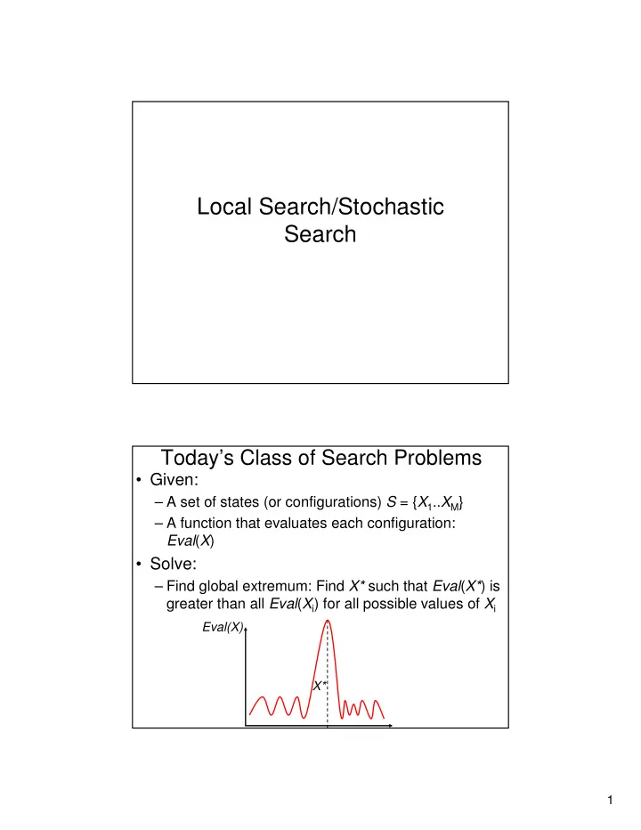
Today’s Class of Search Problems
- Given:
– A set of states (or configurations) S = {X1..XM} – A function that evaluates each configuration: Eval(X)
- Solve:
Local Search/Stochastic Search Todays Class of Search Problems - - PDF document
Local Search/Stochastic Search Todays Class of Search Problems Given: A set of states (or configurations) S = { X 1 .. X M } A function that evaluates each configuration: Eval ( X ) Solve: Find global extremum: Find X*
The definition of the neighborhoods is not
depends critically on the definition of the neihborhood which is not straightforward in general. Ingredient 1. Selection strategy: How to decide which neighbor to accept Ingredient 2. Stopping condition
6 7 2 1 4 8 5 3 1 6 7 2 1 4 8 5 3 6 7 2 1 4 8 5 3 6 7 2 4 5 3 8
Data from: Aarts & Lenstra, “Local Search in Combinatorial Optimization”, Wiley Interscience Publisher
2.1% 1.0% 3-Opt (Best of 1000) 13.7 1.2 3.1% 2.5% 3-Opt 3.6% 1.9% 2-Opt (Best of 1000) 11 1 4.9% 4.5% 2-Opt Running time (N=1000) Running time (N=100) % error from min cost (N=1000) % error from min cost (N=100)
Data from: Aarts & Lenstra, “Local Search in Combinatorial Optimization”, Wiley Interscience Publisher
21 (success)/64 (failure) 94% With sideways moves 4 14% Direct hill climbing Average number of moves % Success N = 8
Data from Russell & Norvig
Select a variable xi at random
Select the variable xi such that changing xi will unsatisfy the least number of clauses (Max of Eval(X))
For more details and useful examples/code: http://www.cs.washington.edu/homes/kautz/walksat/
E = E(X) E’ = E(X’) E = E(X) E’ = E(X’)
Increasing |∆E| Increasing T
Starting point: We move most of the time uphill T = T = Iteration 150: Random downhill moves allow us to escape the local extremum
T = Iteration 180: Random downhill moves have pushed us past the local extremum Iteration 800: As T decreases, fewer downhill moves are allowed and we stay at the maximum T =
– State of solid Configurations X – Energy Evaluation function Eval(.)
Iterations
Iterations Initial Configuration Final configuration after convergence
Iterations Initial Configuration Final configuration after convergence
– The string is the chromosome representing the individual – String made up of genes – Configuration of genes are passed on to offsprings – Configurations of genes that contribute to high fitness tend to survive in the population
– Reproduction: Choose 2 “parents” and produce 2 “offsprings” – Mutation: Choose a random entry in one (randomly selected) configuration and change it
population Y
Generation Cost Minimum cost Average cost in population
Optimal solution reached at generation 35
Initial population Best rN elements in population candidate for reproduction Best (lowest cost) element in population
Population at generation 15 Population at generation 35
Cost Minimum cost Average cost in population
Stabilizes at generation 23
Converges and remains stable after generation 23 0.4% difference: GA = 11.801 SA = 11.751 But: Number of operations (number of cost evaluations) much smaller (approx. 2500)
Population at generation 40
Use genetic algorithms as before with this definition of crossover Example applications: robot controller, signal processing, circuit design Intriguing, but alternative solutions exist for most of these applications; this is not the first approach to consider!!!
http://www.genetic-programming.org/
Population contains
∈
Y s X
– State representation – Neighborhoods – Evaluation function – Additional knowledge and heuristics