4 Local Search For realistic problems, complete search trees can be - - PowerPoint PPT Presentation

T–79.4201 Search Problems and Algorithms

4 Local Search

For realistic problems, complete search trees can be extremely large and difficult to prune effectively. It may often be more useful to get a reasonably good solution fast, rather than the globally optimal one after a long wait. In such cases, local search methods provide an interesting alternative. Assume that the search space X has some neighbourhood structure N, whereby for each solution x ∈ X, a set of “structurally close” solutions N(x) ⊆ X can be easily generated from x by local transformations. For instance, in the case of SAT one could have: N(t) = {truth assignments t′ that differ from t at exactly one variable}, and in the case of SPINGLASS: N(s) = {spin configurations s′ that differ from s at exactly one spin}.

I.N. & P .O. Autumn 2007 T–79.4201 Search Problems and Algorithms

Local search paradigms

◮ Simple local search (iterative improvement) ◮ Simulated annealing ◮ Tabu search ◮ Record-to-record travel ◮ Local search for satisfiability: GSAT, NoisyGSAT, WalkSAT ◮ Other paradigms

I.N. & P .O. Autumn 2007 T–79.4201 Search Problems and Algorithms

4.1 Simple local search (iterative improvement)

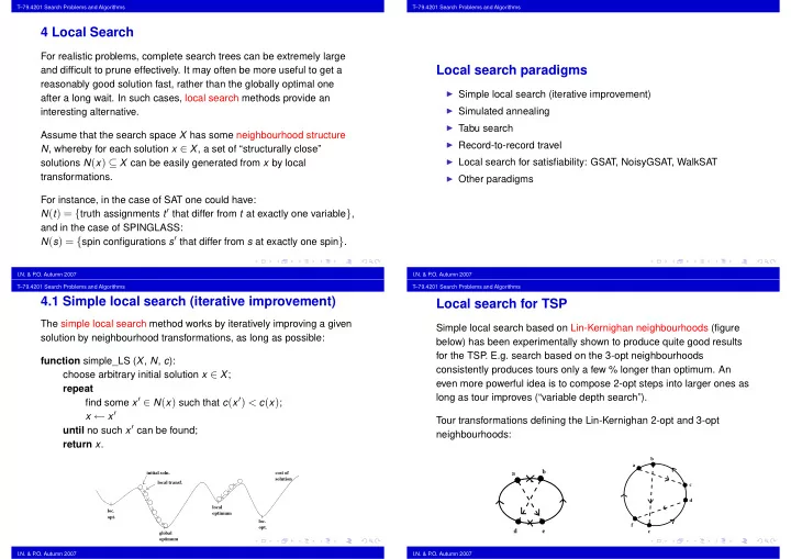
The simple local search method works by iteratively improving a given solution by neighbourhood transformations, as long as possible: function simple_LS (X, N, c): choose arbitrary initial solution x ∈ X; repeat find some x′ ∈ N(x) such that c(x′) < c(x); x ← x′ until no such x′ can be found; return x.

loc.

• pt.

global

• ptimum

local

• ptimum

loc.

• pt.

cost of solution initial soln. local transf.

I.N. & P .O. Autumn 2007 T–79.4201 Search Problems and Algorithms

Local search for TSP

Simple local search based on Lin-Kernighan neighbourhoods (figure below) has been experimentally shown to produce quite good results for the TSP . E.g. search based on the 3-opt neighbourhoods consistently produces tours only a few % longer than optimum. An even more powerful idea is to compose 2-opt steps into larger ones as long as tour improves (“variable depth search”). Tour transformations defining the Lin-Kernighan 2-opt and 3-opt neighbourhoods:

• ✁

a b d e

f e a b d c I.N. & P .O. Autumn 2007

T–79.4201 Search Problems and Algorithms

A 2-Opt descent to local optimum for TSP

I.N. & P .O. Autumn 2007 T–79.4201 Search Problems and Algorithms

4.2 Simulated annealing

Local (nonglobal) minima are obviously a problem for deterministic local search, and many heuristics have been developed for escaping from them. One of the most widely used is simulated annealing (Kirkpatrick, Gelatt & Vecchi 1983, ˇ Cerny 1985), which introduces a mechanism for allowing also cost-increasing moves in a controlled stochastic way. The amount of stochasticity is regulated by a computational temperature parameter T, whose value is during the search decreased from some large initial value Tinit ≫ 0 to some final value Tfinal ≈ 0. A proposed move from a solution x to a worse solution x′ is accepted with probability e−∆c/T , where ∆c > 0 is the cost difference

• f the solutions.

I.N. & P .O. Autumn 2007 T–79.4201 Search Problems and Algorithms

function SA(X, N, c): T ← Tinit; x ← xinit; while T > Tfinal do L ← sweep(T); for L times do choose x′ ∈ N(x) uniformly at random;

∆c ← c(x′)− c(x);

if ∆c ≤ 0 then x ← x′ else choose r ∈ [0,1) uniformly at random; if r ≤ exp(−∆c/T) then x ← x′; end for; T ← lower(T) end while; return x.

I.N. & P .O. Autumn 2007 T–79.4201 Search Problems and Algorithms

Cooling schedules

An important question in applying simulated annealing is how to choose appropriate functions lower(T) and sweep(T), i.e. what is a good “cooling schedule” T0,L0,T1,L1,... There are theoretical results guaranteeing that if the cooling is “sufficiently slow”, then the algorithm almost surely converges to globally optimal solutions. Unfortunately these theoretical cooling schedules are astronomically slow. In practice, it is customary to just start from some “high” temperature T0, and after each “sufficiently long” sweep L decrease the temperature by some “cooling factor” α ≈ 0.8...0.99, i.e. to set Tk+1 = αTk. Theoretically this is much too fast, but often seems to work well

• enough. No one really understands why.

I.N. & P .O. Autumn 2007

T–79.4201 Search Problems and Algorithms

Convergence of simulated annealing

View the search space X with neighbourhood structure N as a graph

(X,N). Assume that this graph is undirected, connected, and of

degree r. (Each node=solution has exactly r neighbours.) Denote by X ∗ ⊆ X the set of globally optimal solutions. The following result was proved by Geman & Geman (1984) and Mitra, Romeo & Sangiovanni-Vincentelli (1986):

I.N. & P .O. Autumn 2007 T–79.4201 Search Problems and Algorithms

• Theorem. Consider a simulated annealing computation on structure

(X,N,c). Assume the neighbourhood graph (X,N) is connected and

regular of degree r. Denote:

∆ = max{c(x′)− c(x) | x ∈ X,x′ ∈ N(x)}.

Choose L ≥ min

x∗∈X∗ max x /

∈X∗ dist(x,x∗),

where dist(x,x∗) is the shortest-path distance in graph (X,N) from node x to node x∗. Suppose the cooling schedule used is of the form

T0,L,T1,L,T2,L,..., where for each cooling stage ℓ ≥ 2:

Tℓ ≥ L∆ lnℓ

(but Tℓ − − →

ℓ→∞ 0).

I.N. & P .O. Autumn 2007 T–79.4201 Search Problems and Algorithms

Then the distribution of states visited by the computation converges in the limit to π∗, where

π∗

x =

• 0,

if x ∈ X \ X ∗,

1/|X ∗|,

if x ∈ X ∗.

I.N. & P .O. Autumn 2007 T–79.4201 Search Problems and Algorithms

4.3 Tabu search (Glover 1986)

Idea: Prevent a local search algorithm from getting stuck at a local minimum, or cycling at a set of solutions with the same objective function value, by maintaining a limited history of recent solutions (tabu list) and excluding those solutions from the move selection process.

I.N. & P .O. Autumn 2007

T–79.4201 Search Problems and Algorithms

function TABU(c, tt): x ← initial feasible solution; initialise TL to {x}; while moves < max_moves do remove from TL solutions entered there more than tt moves ago; choose an x′ ∈ N(x)\ TL of minimum cost; add x to TL; x ← x′ end while; return best x seen so far.

I.N. & P .O. Autumn 2007 T–79.4201 Search Problems and Algorithms

Tabu search: practical considerations

To save tabu list memory and access time, it may be worthwhile not to store complete solutions in the list, but just the recent moves (local transformations). This, however, introduces the problem that a move may be superfluously tabu at time t from the context of some earlier solution xt′, t′ < t, whereas it would lead to an interesting new solution in the context of solution xt. To resolve this issue, heuristics for overriding the tabu rule have been introduced, such as “always accept objective-improving moves” (i.e. such that c(x′) < c(x)).

I.N. & P .O. Autumn 2007 T–79.4201 Search Problems and Algorithms

Tabu search applied to SAT

Given propositional formula F on n variables {x1,...,xn} in conjunctive normal form, choose:

◮ Feasible solutions: truth assignments t : {x1,...,xn} → {0,1}. ◮ Objective function: c(t) = number of clauses in F unsatisfied by

t.

◮ Neighourhood structure: N(t) = truth assignments t′ that differ

from t in exactly one variable.

◮ Full tabu list: recently visited truth assignments. ◮ Abbreviated tabu list: recently flipped variables.

I.N. & P .O. Autumn 2007 T–79.4201 Search Problems and Algorithms

4.4 Record-to-record travel (Dueck 1993)

Idea: Candidate solution can move freely within a tolerance δ of the best (“record”) solution value found so far. When a new record solution is found, the tolerance level falls correspondingly. function RRT(c, δ): x ← initial feasible solution; x∗ ← x; c∗ ← c(x); while moves < max_moves do choose some x′ ∈ N(x); if c(x′) ≤ c∗ +δ then x ← x′; if c(x′) < c∗ then x∗ ← x′; c∗ ← c(x′) end while; return x∗.

I.N. & P .O. Autumn 2007

T–79.4201 Search Problems and Algorithms

RRT applied to SAT

As in tabu search: given propositional formula F on n variables

{x1,...,xn} in conjunctive normal form, choose:

◮ Feasible solutions: truth assignments t : {x1,...,xn} → {0,1}. ◮ Objective function: c(t) = number of clauses in F unsatisfied by

t.

◮ Neighourhood structure: N(t) = truth assignments t′ that differ

from t in exactly one variable.

I.N. & P .O. Autumn 2007 T–79.4201 Search Problems and Algorithms

4.5 Local search for satisfiability: GSAT, NoisyGSAT, WalkSAT GSAT (Gu, Selman et al. 1992)

Idea: View propositional satisfiability as an optimisation problem, where c = cF(t) is the number of unsatisfied clauses in formula F under truth assignment t. Apply the simple (“greedy”) local search strategy to minimise c(t). Note: Because of the greedy descent strategy, the algorithm may get stuck at a local minimum of c(t). To avoid this, the basic algorithm needs to be complemented by some restart rule, tabu list or similar protocol.

I.N. & P .O. Autumn 2007 T–79.4201 Search Problems and Algorithms

function GSAT(F): t ← initial truth assignment; while flips < max_flips do if t satisfies F then return t else find a variable x whose flipping in t causes largest decrease in c(t) (if no decrease is possible, then smallest increase); t ← (t with variable x flipped) end while; return t.

I.N. & P .O. Autumn 2007 T–79.4201 Search Problems and Algorithms

NoisyGSAT (Selman et al. ∼ 1996)

Idea: Augment GSAT by a fraction p of random walk moves. function NoisyGSAT(F,p): t ← initial truth assignment; while flips < max_flips do if t satisfies F then return t else with probability p, pick a variable x uniformly at random; with probability (1− p), do basic GSAT move: find a variable x whose flipping causes largest decrease in c(t) (if no decrease is possible, then smallest increase); t ← (t with variable x flipped) end while; return t.

I.N. & P .O. Autumn 2007

T–79.4201 Search Problems and Algorithms

WalkSAT (Selman et al. 1996)

Idea: NoisyGSAT with the provision that the choice of flipped variables is always focused to the presently unsatisfied clauses.

I.N. & P .O. Autumn 2007 T–79.4201 Search Problems and Algorithms

function WalkSAT(F,p): t ← initial truth assignment; while flips < max_flips do if t satisfies F then return t else choose a random unsatisfied clause C in F; if some variables in C can be flipped without breaking any presently satisfied clauses, then pick one such variable x at random; else: with probability p, pick a variable x in C unif. at random; with probability (1− p), do basic GSAT move: find a variable x in C whose flipping causes largest decrease in c(t); t ← (t with variable x flipped) end while; return t.

I.N. & P .O. Autumn 2007 T–79.4201 Search Problems and Algorithms

WalkSAT vs. NoisyGSAT

The focusing seems to be important: in the (unsystematic) experiments in Selman et al. (1996), WalkSAT outperforms NoisyGSAT by several orders of magnitude. Later experimental evidence by other authors corroborates this. Good values for the “noise” parameter p seem to be about p ≈ 0.5. For instance, for large randomly generated 3-SAT formulas with clauses-to-variables ratio α near the “satisfiability threshold”

α = 4.267, the optimal value of p seems to be about p = 0.57.

By our experiments (Lecture 12), a focused variant of RRT is competitive with WalkSAT on large randomly generated 3-SAT

• instances. What about other focused local search algorithms (e.g.

focused tabu search)?

I.N. & P .O. Autumn 2007 T–79.4201 Search Problems and Algorithms

4.6 Other paradigms

A large number of other local search paradigms have been discussed in the literature, making use of dynamically changing neighbourhood structures, adaptive evaluation functions etc. Classification by Hoos & Stützle (2005):

◮ Iterative improvement (II) ◮ Randomised iterative improvement (RII) ◮ Variable neighbourhood descent (VND) ◮ Variable depth search (VDS) ◮ Simulated annealing (SA) ◮ Tabu search (TS) ◮ Dynamic local search (DLS) ◮ Iterated local search (ILS) ◮ Greedy randomised ’adaptive’ search (GRASP) ◮ Adaptive iterated construction scheme (AICS) ◮ Ant colony optimisation (ACO) ◮ Memetic algorithm (MA)

I.N. & P .O. Autumn 2007