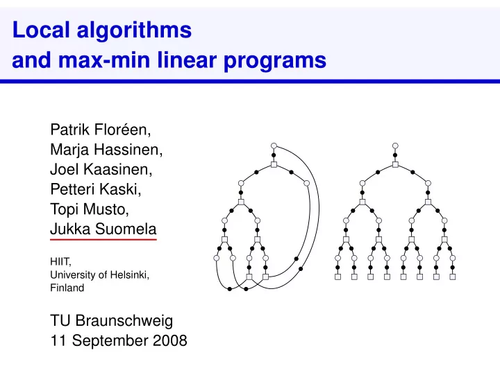
Local algorithms and max-min linear programs Patrik Floren, Marja - - PowerPoint PPT Presentation

Local algorithms and max-min linear programs

Patrik Floréen, Marja Hassinen, Joel Kaasinen, Petteri Kaski, Topi Musto, Jukka Suomela

HIIT, University of Helsinki, Finland

TU Braunschweig 11 September 2008

Local algorithms

Local algorithm: output of a node is a function of input within its constant-radius neighbourhood

(Linial 1992; Naor and Stockmeyer 1995)

2 / 39

Local algorithms

Local algorithm: changes outside the local horizon

• f a node do not affect its output

(Linial 1992; Naor and Stockmeyer 1995)

3 / 39

Local algorithms

Local algorithms are efficient:

◮ Space and time complexity is constant per node ◮ Distributed constant time (even in an infinite network)

. . . and fault-tolerant:

◮ Topology change only affects a constant-size part

(Naor and Stockmeyer 1995)

◮ Can be turned into self-stabilising algorithms

(Awerbuch and Sipser 1988; Awerbuch and Varghese 1991)

(In this presentation, we assume bounded-degree graphs)

4 / 39

Local algorithms

Applications beyond distributed systems:

◮ Simple linear-time centralised algorithm ◮ In some cases randomised, approximate

sublinear-time algorithms

(Parnas and Ron 2007)

Consequences in theory of computing:

◮ Bounded-fan-in, constant-depth Boolean circuits: in NC0 ◮ Insight into algorithmic value of information

(cf. Papadimitriou and Yannakakis 1991)

5 / 39

Local algorithms

Great, but do they exist? Fundamental hurdles:

• 1. Breaking the symmetry:

e.g., colouring a ring of identical nodes

• 2. Non-local problems:

e.g., constructing a spanning tree Strong negative results are known:

◮ 3-colouring of n-cycle not possible,

even if unique node identifiers are given

(Linial 1992)

◮ No constant-factor approximation of vertex cover, etc.

(Kuhn et al. 2004; Kuhn 2005)

6 / 39

Local algorithms

Side information Many positive results are known, if we assume some side information (e.g., coordinates, clustering)

(Czyzowicz et al. 2008; Floréen et al. 2007; Hassinen et al. 2008; Urrutia 2007; Wang and Li 2006; Wiese and Kranakis 2008; . . . )

Side information helps to break the symmetry But what if we have no side information?

7 / 39

Local algorithms

Some previous positive results:

◮ Locally checkable labellings

(Naor and Stockmeyer 1995)

◮ Dominating set

(Kuhn and Wattenhofer 2005; Lenzen et al. 2008)

◮ Packing and covering LPs

(Papadimitriou and Yannakakis 1993; Kuhn et al. 2006)

Present work:

◮ Max-min LPs

(Floréen et al. 2008a,b,c,d)

8 / 39

Max-min linear program

Let A ≥ 0, ck ≥ 0 Objective: maximise min

k∈K ck · x

subject to A x ≤ 1, x ≥ 0 Generalisation of packing LP: maximise c · x subject to A x ≤ 1, x ≥ 0

9 / 39

Max-min linear program

Let A ≥ 0, C ≥ 0 Equivalent formulation: maximise

ω

subject to A x ≤ 1, C x ≥ ω1, x ≥ 0 Applications: mixed packing and covering, linear equations find x s.t. A x ≤ 1, find x s.t. A x = 1, C x ≥ 1, x ≥ 0 x ≥ 0

10 / 39

Max-min linear program

Distributed setting:

◮ one node v ∈ V for each variable xv,

• ne node i ∈ I for each constraint ai · x ≤ 1,
• ne node k ∈ K for each objective ck · x

◮ v ∈ V and i ∈ I adjacent if aiv > 0,

v ∈ V and k ∈ K adjacent if ckv > 0 maximise min

k∈K ck · x

subject to A x ≤ 1, x ≥ 0

11 / 39

Max-min linear program

Distributed setting:

◮ one node v ∈ V for each variable xv,

• ne node i ∈ I for each constraint ai · x ≤ 1,
• ne node k ∈ K for each objective ck · x

◮ v ∈ V and i ∈ I adjacent if aiv > 0,

v ∈ V and k ∈ K adjacent if ckv > 0 Key parameters:

◮ ∆I = max. degree of i ∈ I ◮ ∆K = max. degree of k ∈ K

12 / 39

Example

Task: Data gathering in a sensor network

◮ circle = sensor ◮ square = relay ◮ edge = network connection

13 / 39

Example

Task: Maximise the minimum amount of data gathered from each sensor maximise min { x1, x2 + x4, x3 + x5 + x7, x6 + x8, x9

}

1 2 3 7 8 9 4 5 6

14 / 39

Example

Task: Maximise the minimum amount of data gathered from each sensor; each relay has a limited battery capacity maximise min { x1, x2 + x4, x3 + x5 + x7, x6 + x8, x9

}

subject to x1 + x2 + x3 ≤ 1, x4 + x5 + x6 ≤ 1, x7 + x8 + x9 ≤ 1, x1, x2, . . . , x9 ≥ 0

1 2 3 7 8 9 4 5 6

15 / 39

Example

Task: Maximise the minimum amount of data gathered from each sensor; each relay has a limited battery capacity An optimal solution: x1 = x5 = x9 = 3/5, x2 = x8 = 2/5, x4 = x6 = 1/5, x3 = x7 = 0

1 2 3 7 8 9 4 5 6

16 / 39

Example

Communication graph:

G = (V ∪ I ∪ K, E)

maximise min { x1, x2 + x4, x3 + x5 + x7, x6 + x8, x9

}

subject to x1 + x2 + x3 ≤ 1, x4 + x5 + x6 ≤ 1, x7 + x8 + x9 ≤ 1, x1, x2, . . . , x9 ≥ 0

k ∈ K i ∈ I v ∈ V

17 / 39

Example

Communication graph:

G = (V ∪ I ∪ K, E)

maximise min { x1, x2 + x4, x3 + x5 + x7, x6 + x8, x9

}

subject to x1 + x2 + x3 ≤ 1, x4 + x5 + x6 ≤ 1, x7 + x8 + x9 ≤ 1, x1, x2, . . . , x9 ≥ 0

k ∈ K i ∈ I v ∈ V

18 / 39

Example

Communication graph:

G = (V ∪ I ∪ K, E)

maximise min { x1, x2 + x4, x3 + x5 + x7, x6 + x8, x9

}

subject to x1 + x2 + x3 ≤ 1, x4 + x5 + x6 ≤ 1, x7 + x8 + x9 ≤ 1, x1, x2, . . . , x9 ≥ 0

k ∈ K i ∈ I v ∈ V

19 / 39

Old results

“Safe algorithm”: Node v chooses xv = min

i : aiv>0

1 aiv |{u : aiu > 0}|

(Papadimitriou and Yannakakis 1993)

Factor ∆I approximation Uses information only in radius 1 neighbourhood of v A better approximation ratio with a larger radius?

20 / 39

New results, general case

The safe algorithm is factor ∆I approximation Theorem For any ǫ > 0, there is a local algorithm for max-min LPs with approximation ratio ∆I (1 − 1/∆K) + ǫ Theorem There is no local algorithm for max-min LPs with approximation ratio ∆I (1 − 1/∆K)

Degree of a constraint i ∈ I is at most ∆I Degree of an objective k ∈ K is at most ∆K

21 / 39

New results, bounded growth

Assume bounded relative growth beyond radius R:

|B(v, r + 2)| |B(v, r)| ≤ 1 + δ

for all v ∈ V, r ≥ R where B(v, r) = agents in radius r neighbourhood of v Theorem There is a local algorithm for max-min LPs with approximation ratio 1 + 2δ + o(δ) There is no local algorithm for max-min LPs with approximation ratio 1 + δ/2

(assuming ∆I ≥ 3, ∆K ≥ 3, 0.0 < δ < 0.1)

22 / 39

Approximability, bounded growth

Step 1: Choose local constant-size subproblems Step 3: Solve them optimally Step 3: Take averages of local solutions, add some slack

23 / 39

Approximability, general case

Preliminary step 1: Unfold the graph into an infinite tree

a b c d a b c c b d a d a b c c a b d b a c c a d b d a c b a c b d d

24 / 39

Approximability, general case

Preliminary step 2: Apply a sequence of local transformations (and unfold again)

→ → → →

25 / 39

Approximability, general case

It is enough to design a local approximation algorithm for the following special case:

◮ Communication graph G is an (infinite) tree ◮ Degree of each constraint i ∈ I is exactly 2 ◮ Degree of each objective k ∈ K is at least 2 ◮ Each agent v ∈ V adjacent to at least one constraint ◮ Each agent v ∈ V adjacent to exactly one objective ◮ ckv ∈ {0, 1}

26 / 39

Approximability, general case

After the local transformations, we have an infinite tree with a fairly regular structure In a centralised setting, we could organise the nodes into layers Then we could design an approximation algorithm. . .

27 / 39

Approximability, general case

“Switch off” every Rth layer of objectives

28 / 39

Approximability, general case

“Switch off” every Rth layer of objectives Consider all possible locations (shifting strategy)

29 / 39

Approximability, general case

“Switch off” every Rth layer of objectives Consider all possible locations (shifting strategy)

30 / 39

Approximability, general case

“Switch off” every Rth layer of objectives Consider all possible locations (shifting strategy) Solve the LP for the “active” layers, take averages Factor R/(R − 1) approximation

31 / 39

Approximability, general case

We could solve the LP simply by propagating information upwards between a pair of “passive” layers But we cannot choose the layers by any local algorithm! Two fundamentally different roles for agents: “up” and “down” How to choose the roles? How to break the symmetry?

32 / 39

Approximability, general case

Trick: consider both possible roles for each agent, “up” an “down” Compute locally two candidate solutions, one for each role Take averages Surprise: factor ∆I (1 − 1/∆K) + ǫ approximation, best possible!

33 / 39

Approximability, general case

Some complications:

◮ several optimal solutions ◮ how to make sure that

the local choices are “compatible” with each other? Key idea:

◮ “down” nodes choose

as large values as possible

◮ “up” nodes choose

as small values as possible

34 / 39

Inapproximability

Regular high-girth graph or regular tree?

35 / 39

Inapproximability

Locally indistinguishable

36 / 39

Inapproximability

Optimum ≤ 2/3 vs. optimum ≥ 1

1 3 1 3 1 3 1 3 1 3 1 3 1 3 1 3 1 3 1 3 1 3 1 3 1 3 1 3 1 3 1 3 1 3 1 3

1 1 1 1 1 1 1 1 1 1 1 1 1 1 1

37 / 39

Inapproximability

• Approx. ratio ≥ 1/(2/3) = 3 (1 − 1/2) = ∆I (1 − 1/∆K)

1 3 1 3 1 3 1 3 1 3 1 3 1 3 1 3 1 3 1 3 1 3 1 3 1 3 1 3 1 3 1 3 1 3 1 3

1 1 1 1 1 1 1 1 1 1 1 1 1 1 1

38 / 39

Summary

Max-min linear programs: given A, ck ≥ 0, maximise min

k∈K ck · x

subject to A x ≤ 1, x ≥ 0 Local algorithms: output of a node is a function of input within its constant-radius neighbourhood Main result: tight characterisation of local approximability

http://www.hiit.fi/ada/geru — jukka.suomela@cs.helsinki.fi

39 / 39

References (1)

• B. Awerbuch and M. Sipser (1998). Dynamic networks are as fast as

static networks. FOCS 1988. [DOI]

• B. Awerbuch and G. Varghese (1991). Distributed program checking:

a paradigm for building self-stabilizing distributed protocols. FOCS 1991. [DOI]

• J. Czyzowicz, S. Dobrev, T. Fevens, H. González-Aguilar, E. Kranakis,
• J. Opatrny, and J. Urrutia (2008). Local algorithms for dominating and

connected dominating sets of unit disk graphs with location aware

• nodes. LATIN 2008. [DOI]

P . Floréen, P . Kaski, T. Musto, and J. Suomela (2007). Local approximation algorithms for scheduling problems in sensor networks. ALGOSENSORS 2007. [DOI] P . Floréen, P . Kaski, T. Musto, and J. Suomela (2008a). Approximating max-min linear programs with local algorithms. IPDPS 2008. [DOI]

References (2)

P . Floréen, M. Hassinen, P . Kaski, and J. Suomela (2008b). Local approximation algorithms for a class of 0/1 max-min linear programs. Manuscript, arXiv:0806.0282 [cs.DC]. P . Floréen, M. Hassinen, P . Kaski, and J. Suomela (2008c). Tight local approximation results for max-min linear programs. ALGOSENSORS 2008. P . Floréen, J. Kaasinen, P . Kaski, and J. Suomela (2008d). An optimal local approximation algorithm for max-min linear programs. Manuscript, arXiv:0809.1489 [cs.DC].

• M. Hassinen, V. Polishchuk, and J. Suomela (2008). Local

3-approximation algorithms for weighted dominating set and vertex cover in quasi unit-disk graphs. LOCALGOS 2008.

• F. Kuhn (2005). The Price of Locality: Exploring the Complexity of

Distributed Coordination Primitives. PhD thesis.

References (3)

• F. Kuhn and R. Wattenhofer (2005). Constant-time distributed dominating

set approximation. Distributed Computing, 17(4):303–310. [DOI]

• F. Kuhn, T. Moscibroda, and R. Wattenhofer (2004).

What cannot be computed locally! PODC 2004. [DOI]

• F. Kuhn, T. Moscibroda, and R. Wattenhofer (2006).

The price of being near-sighted. SODA 2006. [DOI]

• C. Lenzen, Y. A. Oswald, and R. Wattenhofer (2008).

What can be approximated locally? SPAA 2008.

• N. Linial (1992). Locality in distributed graph algorithms.

SIAM Journal on Computing, 21(1):193–201. [DOI]

• M. Naor and L. Stockmeyer (1995). What can be computed locally?

SIAM Journal on Computing, 24(6):1259–1277. [DOI]

References (4)

• C. H. Papadimitriou and M. Yannakakis (1991). On the value of

information in distributed decision-making. PODC 1991. [DOI]

• C. H. Papadimitriou and M. Yannakakis (1993).

Linear programming without the matrix. STOC 1993. [DOI]

• M. Parnas and D. Ron (2007). Approximating the minimum vertex cover

in sublinear time and a connection to distributed algorithms. Theoretical Computer Science, 381(1–3):183–196. [DOI]

• J. Urrutia (2007). Local solutions for global problems in wireless
• networks. Journal of Discrete Algorithms, 5(3):395–407. [DOI]
• Y. Wang and X.-Y. Li (2006). Localized construction of bounded degree

and planar spanner for wireless ad hoc networks. Mobile Networks and Applications, 11(2):161–175. [DOI]

• A. Wiese and E. Kranakis (2008). Local PTAS for independent set and

vertex cover in location aware unit disk graphs. DCOSS 2008. [DOI]