
SLIDE 1
Linear functors and modal logic
R.A.G. Seely
John Abbott College & McGill University
1
- An extension of an idea from a paper [Blute, Cockett, Seely;
MSCS 2002] – Modal logic given by a linear functor (a special case of “the logic of linear functors”)
- Based on an “abandoned” project [Sadrzadeh, Cockett, Seely,
2009–2010, intended for MFPS 2010] – Adjoint modal pairs (think two varieties of “possibly” and “necessarily”) (as given in “positive tense logic” of Prior) – Relational models of such modal logic (using some ideas
- f Hermida, IMLA 2002)
2
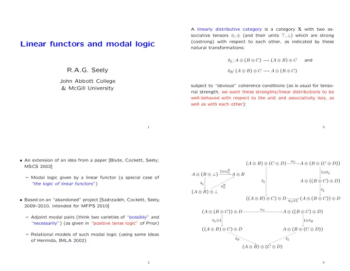
A linearly distributive category is a category X with two as- sociative tensors ⊗, ⊕ (and their units ⊤, ⊥) which are strong (costrong) with respect to each other, as indicated by these natural transformations: δL: A ⊗ (B ⊕ C) − → (A ⊗ B) ⊕ C and δR: (A ⊕ B) ⊗ C − → A ⊕ (B ⊗ C) subject to “obvious” coherence conditions (as is usual for tenso- rial strength, we want these strengths/linear distributions to be well-behaved with respect to the unit and associativity isos, as well as with each other):
3
A ⊗ (B ⊕ ⊥)
1⊗uR
⊕
δL
- A ⊗ B
(A ⊗ B) ⊕ ⊥
uR
⊕
- (A ⊗ B) ⊗ (C ⊕ D)
a⊗
- δL
- A ⊗ (B ⊗ (C ⊕ D))
1⊗δL
- A ⊗ ((B ⊗ C) ⊕ D)
δL
- ((A ⊗ B) ⊗ C) ⊕ D a⊗⊕1
(A ⊗ (B ⊗ C)) ⊕ D
(A ⊗ (B ⊕ C)) ⊗ D
a⊗
- δL⊗1
- A ⊗ ((B ⊕ C) ⊗ D)
1⊗δR
- ((A ⊗ B) ⊕ C) ⊗ D
δR
- A ⊗ (B ⊕ (C ⊗ D))
δL
- (A ⊗ B) ⊕ (C ⊗ D)
4