LECTURE 4: Growth, TFP, Domestic and International Capital Flows - - PowerPoint PPT Presentation

LECTURE 4: Growth, TFP, Domestic and International Capital Flows with Other Frictions in Financial Intermediation: Costly State Verification, Adverse Selection, and Moral Hazard Cross-country in steady state, and an example of unbalanced growth

1

Greenwood, Sanchez, and Wang (2013),“Quantifying the Impact of Financial Development on Economic Development”

A model which is meant to capture Levine’s review of the first lecture, that is, a particular function of financial intermediation, and technological progress in that intermediation, incorporated into a growth model. Address cross-country interest rates spreads and a resource-using costly state verification with diminishing returns and exogenous technological progress. Uganda could more than double its output if it would adopt best practice in financial sector (maximum technology available world-wide). However, this is still only 29% of the gap between its potential and actual output). In the model, improvements in financial intermediation account for 29% of U.S. growth. The framework also is capable of mimicking the striking decline in the Taiwanese interest-rate spread. At the same time, it predicts a significant rise in its capital-to-output ratio. It is estimated that dramatic improvements in Taiwans financial sector accounted for 45% of the country’s economic growth.

2

Greenwood, Sanchez, and Wang (2013),“Quantifying the Impact of Financial Development on Economic Development”

• Fig. 1. Interest-rate spreads and capital-to-GDP ratios for the United States and Taiwan, 1970–2005. Data sources for all figures are discussed in Appendix A.

3

Greenwood, Sanchez, and Wang (2013),“Quantifying the Impact of Financial Development on Economic Development”

Levine (2005), King and Levine (1993): the upshot is that financial development has a causal effect on economic development; specifically, it leads to higher rates of growth in income and productivity. We investigate this impact quantitatively, using a costly state verification

• model. The source of inspiration for the framework is the classic work by

Townsend (1979) and Williamson (1986).

Novel twists:

• 1. Firms monitor cash flows; however, here the efficiency of this activity

depends on both the amount of resources devoted to it and the productivity of the monitoring technology used in the financial sector.

• 2. Firms have ex-ante differences in the structure of returns that they offer.

4

Greenwood, Sanchez, and Wang (2013),“Quantifying the Impact of Financial Development on Economic Development”

A financial theory of firm size emerges:

◮ At any point in time, firms offering high expected returns are underfunded

(relative to a world without informational frictions), whereas others yielding low expected returns are overfunded. This results from diminishing returns in information production.

◮ As the efficiency of the financial sector rises (relative to the rest of the

economy), funds are redirected away from less productive firms in the economy toward more productive ones.

◮ As the interest-rate spread declines and the cost of borrowing falls, capital

deepening occurs in the economy.

5

Greenwood, Sanchez, and Wang (2013),“Quantifying the Impact of Financial Development on Economic Development”

• Fig. 2. The cross-country relationship among interest-rate spreads, capital-to-GDP ratios and GDPs per capita. The three letter country codes are taken from

the International Organization for Standardization, ISO 3166-1 alpha-3.

6

Greenwood, Sanchez, and Wang (2013),“Quantifying the Impact of Financial Development on Economic Development”

• Fig. 3. The cross-country relationship among interest-rate spreads, TFPs and GDPs per capita.

7

Greenwood, Sanchez, and Wang (2013),“Quantifying the Impact of Financial Development on Economic Development”

Firms:

◮ Firms hire capital, k, and labor, l, to produce output, o, in line with the

constant-returns-to-scale production function o = xθkαl1−α.

◮ The productivity level of a firms production process is represented by xθ,

where x is aggregate and θ is idiosyncratic. The idiosyncratic level of productivity is a random variable. The realized value of θ is drawn from the two-point set τ = {θ1, θ2}, with θ1 < θ2. The set τ is the firms type and differs across firms.

Financial intermediaries:

◮ Intermediation is competitive. ◮ Intermediaries raise funds from consumers and lend them to firms. ◮ Even though an intermediary knows a firms type, τ, it cannot observe the

state of a firms business (θ , o, and l) either costlessly or perfectly.

8

Greenwood, Sanchez, and Wang (2013),“Quantifying the Impact of Financial Development on Economic Development”

Let Pij(lmj, k, z) denote the probability that the firm is caught cheating conditional on the following:

• 1. The true realization of productivity is θi
• 2. The firm makes a report of θj
• 3. The intermediary allocates lmj units of labor to monitor the claim
• 4. The size of the loan is k (which represents the scale of the project)
• 5. The level of productivity in the monitoring activity is z

The function Pij(lmj, k, z) is increasing in lmj and z and decreasing in k. The steady state for the model provides a mapping between productivity in the production (x) and financial sectors (z) on the one hand, and output (o) and interest-rate spreads (s) on the other. This mapping can be inverted to infer x and z using observations on o and s, given a vector of parameter values, p. Take the parameter vector p that was calibrated/estimated for the U.S. economy and use the Taiwanese data on per-capita GDPs and interest-rate spreads for the years 1974 and 2004 to obtain the imputed Taiwanese technology vector.

9

Martin and Taddei (2012), “International Capital Flows and Credit Market Imperfections: a Tale of Two Frictions”

Excessive capital flows and boom-bust cycles (at least in theory, not quantitative/calibrated). In recent years, global imbalances large and persistent capital flows from Asia to the United States and other developed economies have spurred renewed interest in the macroeconomic effects of financial frictions. Financial frictions have also been invoked to explain the run-up to the financial crisis of 2007-08 and the unfolding of events during the crisis itself.

10

Martin and Taddei (2012), “International Capital Flows and Credit Market Imperfections: a Tale of Two Frictions”

Instead of limiting the amount of resources that can be channeled towards productive investment, financial frictions are portrayed in the literature as the source of an excessive supply of assets that has channeled too many resources towards unproductive investment. (We covered such papers earlier, as on China.) We need to acknowledge that there are different types of frictions. On the one hand, underprovision of assets and limited investment are typically attributed to limited pledgeability. On the other hand, overprovision of assets is typically attributed to some form of asymmetric information regarding the quality of borrowers, which fuels investment by unproductive or inefficient individuals. Existing macroeconomic models focus mostly on limited pledgeability while neglecting adverse selection (see previous lecture).

11

Martin and Taddei (2012), “International Capital Flows and Credit Market Imperfections: a Tale of Two Frictions”

We have a standard growth model in which credit markets intermediate resources between savers and investors in capital accumulation. Individuals are endowed with some resources and an investment project for producing capital, and they must decide whether: (i) to undertake their project and become entrepreneurs, in which case they demand funds from credit markets, or; (ii) to forego their project and become savers, in which case they supply their resources to credit markets. To give adverse selection a central role in credit markets, we also assume that an individual’s productivity is private information and thus unobservable by

• lenders. This induces cross-subsidization between high- and low-productivity

entrepreneurs. All borrowers must pay the same contractual interest rate in equilibrium. This implies that high-productivity entrepreneurs, who repay often, effectively face a higher cost of funds than low-productivity entrepreneurs, who repay only

• seldom. It is this feature that gives rise to adverse selection by providing some

low-productivity individuals, who would be savers in the absence of cross-subsidization, with incentives to become entrepreneurs.

12

Martin and Taddei (2012), “International Capital Flows and Credit Market Imperfections: a Tale of Two Frictions”

Macroeconomic implications of adverse selection:

• 1. It leads to an increase in the economy’s equilibrium interest rate, while

boosting equilibrium borrowing and investment.

• 2. By fostering inefficient entrepreneurship, it generates a negative wedge

between the marginal return to investment and the equilibrium interest rate. Through (1), adverse selection induces the economy to attract more capital flows and boosts net capital inflows from the international financial market, relative to the full-information economy. By (2), since the true marginal return to investment lies below the world interest rate, these capital inflows can lead to a fall in aggregate consumption.

13

Moll, Townsend, and Zhorin (2012), “Entrepreneurship, Inequality, and Growth with Information Constrained Factor Markets”

There is evidence that even within a given economy, obstacles to trade may vary depending on location. In a companion paper, Karaivanov and Townsend (2012) estimate the financial/information regime in place for households including those running businesses using Townsend Thai data from rural areas (villages) and from urban areas (towns and cities). They find differences across these locations. For example, a moral hazard constrained financial regime fits best in urban areas and a more limited savings regime in rural areas. More generally, there seems to be (related) regional variation. A number of recent papers argue that financial frictions arising from limited commitment problems can explain large cross-country income differences. We argue that different micro financial underpinnings have potentially very different implications at both the macro and the micro level. To this end, we develop a general equilibrium framework that encompasses different regimes of frictions, and compare the implications of two concrete frictions: limited commitment and moral hazard.

14

Moll, Townsend, and Zhorin (2012), “Entrepreneurship, Inequality, and Growth with Information Constrained Factor Markets”

• 1. Aggregate TFP in the two regimes is depressed but for completely

different reasons:

◮ Under limited commitment this results from a misallocation of capital

across firms with given productivities.

◮ Under moral hazard, TFP is endogenously lower at the firm level because

entrepreneurs exert suboptimal effort.

• 2. Occupational choice, the firm productivity and size distributions, and

income and wealth inequality also differ markedly.

• 3. Individual transitions are much faster in the limited commitment regime

than under the moral hazard, resulting for example in more dispersed wealth growth rates:

◮ In the limited commitment regime binding borrowing constraints and high

marginal products of capital provide an incentive for entrepreneurs to attempt to save themselves out of these constraints.

◮ Under moral hazard individual wealth or promised utility moves slowly as

• utput-dependent penalties and awards are spread into the future.
• 4. There are implications as well for regional and sectoral capital flows.

15

Moll, Townsend, and Zhorin (2012), “Entrepreneurship, Inequality, and Growth with Information Constrained Factor Markets”

In particular, the most realistic financial regime for the given economy, which varies regionally and in urban vs. rural stratifications of the data, is a not a simple convex combination of the two extremes. The bottom line is that the behavior of macro aggregates depends on micro financial underpinnings.

16

Motivation Model Limited Commitment vs. Private Information Mixtures Transitions

Finance and Development:

Limited Commitment vs. Moral Hazard

Benjamin Moll Robert M. Townsend Victor Zhorin Princeton MIT Chicago

17

Motivation Model Limited Commitment vs. Private Information Mixtures Transitions

Motivation

• Micro evidence: even within given economy, obstacles to trade

may vary depending on location.

• For example, ? using Townsend Thai data: moral hazard

constrained financial regime fits best in urban areas and a more limited savings regimes in rural areas.

• More generally, regional variation: ??

18

Motivation Model Limited Commitment vs. Private Information Mixtures Transitions

What We Do

• Ask: What difference do the micro financial foundations make

for the macro economy? Will argue: a big one.

• Develop a general equilibrium model of entrepreneurship and

financial frictions that is general enough to encompass: (1) financial frictions stemming from limited commitment. (2) financial frictions stemming from private information (moral hazard). (3) Mixtures of different regimes in different regions.

19

Motivation Model Limited Commitment vs. Private Information Mixtures Transitions

What We Do

• Study aggregates: GDP, TFP, capital accumulation, wages

and interest rates...

• ...but also micro moments: prod. distribution, size

distribution of firms, dispersion in MPKs.

• Show: all of these look potentially very different, depending
• n the underlying financial regime.

20

Motivation Model Limited Commitment vs. Private Information Mixtures Transitions

Implications for Literature

• Large literature studies role of financial market imperfections

in development.

• Most existing studies: limited commitment.
• Much fewer: moral hazard (???)
• We should use micro data to choose between the myriad of

alternative forms of introducing a financial friction into our models.

21

Motivation Model Limited Commitment vs. Private Information Mixtures Transitions

Common Theoretical Framework

• Households: wealth, a, entrepreneurial ability, z. Markov

process µ(z'|z).

• Continuum of households of measure one, indexed by i ∈ [0, 1]
• Preferences over consumption and effort:

∞

βt E0 u(cit , eit ).

t=0

• Occupational choice: entrepreneur (x = 1) or worker (x = 0).

22

Motivation Model Limited Commitment vs. Private Information Mixtures Transitions

Entrepreneurs and Workers

• Entrepreneurs, x = 1: technologies

y = f (z, ε, k, l) = zεkαlγ , α + γ < 1

• ε ≡ idiosyncratic production risk, with distribution p(ε|e).
• Workers, x = 0: supply ε efficiency units of labor, with

distribution p(ε|e).

• Note: Depending on x = 0 or x = 1, ε is either firm

productivity or worker’s efficiency units. Allow for differential responsiveness to e through appropriate scaling.

23

Motivation Model Limited Commitment vs. Private Information Mixtures Transitions

Risk-Sharing

• Households contract with risk-neutral intermediaries to form

“risk-sharing syndicates”: intermediaries bear some of HH risk.

• “Risk-sharing syndicates” take (w, r) as given.
• Assume: can only insure against production risk, ε, but not

against talent, z.

• Optimal contract:

(1) assigns occupation, x, effort, e, capital, k, and labor, l. After ε is drawn, assigns consumption and savings c(ε) and a

' (ε).

(2) leaves zero profits to intermediary ⇔ maximizes individual’s utility.

24

Motivation Model Limited Commitment vs. Private Information Mixtures Transitions

Timing

25

Motivation Model Limited Commitment vs. Private Information Mixtures Transitions

Optimal Contract: Bellman Equation

v(a, z) = max p(ε|e) {u[c(ε), e] + βEv[a'(ε), z']} s.t.

e,x,k,l,c(ε),a!(ε) ε

p(ε|e) {c(ε) + a'(ε)}

ε 0

≤ p(ε|e) {x[zεkαlγ − wl − (r + δ)k] + (1 − x)wε]} + (1 + r)a

ε

and s.t. regime-specific constraints

Capital Accumulation 26

Motivation Model Limited Commitment vs. Private Information Mixtures Transitions

Private Information

• effort, e, unobserved ⇒ moral hazard problem.
• Note: moral hazard for both entrepreneurs and workers.
• IC constraint:

p(ε|e) u[c(ε), e] + βEv[a

' (ε), z ' ] ε

≥ p(ε|e ˆ) u[c(ε), e ˆ] + βEv[a

' (ε), z ' ]

∀e, e ˆ, x

ε

• Lotteries

Connection to Optimal Dynamic Contract 27

Motivation Model Limited Commitment vs. Private Information Mixtures Transitions

Formulation with Lotteries

Return

• Notation: control variables d = (c, ε, e, x).
• Lotteries: π(d, a

' |a, z) = π(c, ε, e, x, a ' |a, z)

'

v(a, z) = max π(d, a

' |a, z) {u(c, e) + βEv(a , z ' )}

s.t.

π(d,a!|a,z) D,A '

π(d, a

' |a, z) {a + c} D,A

= π(d, a

' |a, z) {xΠ(ε, e, z; w, r) + (1 − x)wε} (1 + r)a. D,A '

π(d, a

' |a, z) {u(c, e) + βEv(a , z ' )} (D\E ),A

p(ε|e ˆ)

'

≥ π(d, a

' |a, z)

{u(c, e ˆ) + βEv(a , z

' )} ∀e, e

ˆ, x p(ε|e)

(D\E ),A

π(d, a

' |a, z) = p(ε|e)

π(d, a

' |a, z),

∀ε, e, x

C ,A C,ε,A

28

Motivation Model Limited Commitment vs. Private Information Mixtures Transitions

Limited Commitment

• effort, e, observed ⇒ perfect insurance against production

risk, ε.

• But collateral constraint:

k ≤ λa, λ ≥ 1.

29

Motivation Model Limited Commitment vs. Private Information Mixtures Transitions

Factor Demands

• Denote optimal occupational choice and factor demands by

x(a, z), l(a, z; w, r), k(a, z; w, r)

• and individual (average) labor supply:

n(a, z; w, r) ≡ [1 − x(a, z)] p[ε|e(a, z)]ε.

ε

30

Motivation Model Limited Commitment vs. Private Information Mixtures Transitions

Steady State Equilibrium

• Prices r and w, and corresponding quantities such that:

(i) Taking as given r and w, quantities are determined by optimal contract (ii) Markets clear l(a, z; w, r)dG (a, z) = n(a, z; w, r)dG (a, z) k(a, z; w, r)dG (a, z) = adG (a, z).

31

Motivation Model Limited Commitment vs. Private Information Mixtures Transitions

Parameterization

• Preferences

1−σ

c χ

1+ϕ

u(c, e) = U(c)−V (e), U(c) = , V (e) = e 1 − σ 1 + ϕ

• Recall production function εzkαlγ .
• Parameters:

α = 0.3, γ = 0.4, δ = 0.06 β = 1.05−1 , σ = 1.5, χ = .5, ϕ = .2 ⎡ ⎤ 0.8 0.2 ⎣ ⎦ ε ∈ {2, 4}, e ∈ {0, 1}, p(ε|e) = 0.2 0.8

• Parameters same (range) as those estimated from micro data

by ?

32

Motivation Model Limited Commitment vs. Private Information Mixtures Transitions

Limited Commitment vs. Moral Hazard

• Savings behavior very different in two regimes.
• Limited commitment: borrowing constrained.

U

' (cit ) = βEz,t

• U

' (cit+1)(1 + r) + µit+1λ

• U

' (cit ) > β(1 + r)Ez,t U ' (cit+1)

33

Motivation Model Limited Commitment vs. Private Information Mixtures Transitions

Limited Commitment vs. Moral Hazard

• Moral hazard: inverse Euler equation (???).
• −1

U

' (cit ) = β(1 + r)Ez,t

Eε,t 1 U

' (cit+1)

• Jensen ⇒ savings constrained

U

' (cit ) < β(1 + r)Ez,t Eε,t U ' (cit+1).

• Note: presence of uninsurable ability z.
• Difference in savings reflected in equilibrium r among others.

34

Motivation Model Limited Commitment vs. Private Information Mixtures Transitions

Limited Commitment vs. Moral Hazard

Table: Comparison of Different Regimes

!"#"$%&'()##"$#%*$ +),-.'/-0-,& 123'45')6'789 :;<=> :;=<: ?73'45')6'789 :;=@@ :;A:B (-C"$-.DEF$CF$'G-$")'45)6'789 :;=BH I;:>I !-J),'KFCC.L'45')6'789 I;:<= :;AA: M%.6-,%'45')6'789 :;NAH :;=== M-O%'45)6'789 :;<BN :;=<@ P*$%,%Q$'G-$% D:;:HI :;:I: 5'R*$,%C,%*%F,Q :;BB< :;IH> RS$%,*-.'7"*-*T%U123 I;H@= >;BAN

35

Motivation Model Limited Commitment vs. Private Information Mixtures Transitions

Limited Commitment vs. Moral Hazard

Figure: Wealth Lorenz Curves

0.1 0.2 0.3 0.4 0.5 0.6 0.7 0.8 0.9 1 0.1 0.2 0.3 0.4 0.5 0.6 0.7 0.8 0.9 1 Limited Commitment Moral Hazard

It can be seen that wealth inequality in higher in the limited commitment regime. This is a direct consequence of the bigger dispersion in marginal products of capital.

36

Motivation Model Limited Commitment vs. Private Information Mixtures Transitions

Mixtures of Moral Hazard and Limited Commitment

• Combine the two regimes in one economy. 50% of pop.

subject to moral hazard, 50% to limited commitment.

• Motivation: no reason why economy as a whole should be

subject to only one friction.

• Estimated “on the ground” by ? and ?: for Thailand, MH fits

better in and around Bangkok and LC better in Northeast (see also ?)

• Also: factor prices different in two regimes ⇒ potentially

interesting GE effects.

37

Motivation Model Limited Commitment vs. Private Information Mixtures Transitions

Mixtures of Moral Hazard and Limited Commitment

Figure: Aggregate Impact of Importance of Moral Hazard vs. Limited Commitment, m

GDP TFP Capital-Output Ratio

0.2 0.4 0.6 0.8 1 0.78 0.8 0.82 0.84 0.86 0.88 Fraction of Population Subject to Moral Hazard, m GDP (% of First−Best) 0.2 0.4 0.6 0.8 1 0.86 0.87 0.88 0.89 0.9 0.91 0.92 Fraction of Population Subject to Moral Hazard, m TFP (% of First−Best) 0.2 0.4 0.6 0.8 1 0.8 0.85 0.9 0.95 1 1.05 Fraction of Population Subject to Moral Hazard, m Capital−Output Ratio (% of First−Best)

Labor Supply

0.2 0.4 0.6 0.8 1 0.98 1 1.02 1.04 1.06 1.08 1.1 Fraction of Population Subject to Moral Hazard, m Labor Supply (% of First−Best)

38

Motivation Model Limited Commitment vs. Private Information Mixtures Transitions

Mixtures of Moral Hazard and Limited Commitment

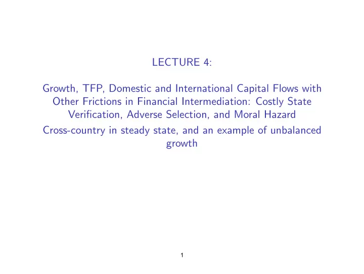
Table: Comparison of LC and MH Sectors in Mixed Regime

!"#$%&'$(")$*&)+,-. /0&1$2345 !6&1$2345 789&:;&4<&=>? ,-@AB ,-AA. C-,.D E=9&:;&4<&=>? ,-D,A ,-DAF ,-D,. 0GH"3GIJKL3HL3&'G3"4&:;4<&=>? ,-D.B ,-A,, C-CMB /GN45&OLHHIP&:;&4<&=>? C-,BQ ,-M@D C-B.@ R$I<G5$&:;&4<&=>? ,-@FC ,-M@M ,-@MA RG($&:;4<&=>? ,-@QC ,-@QC ,-@QC ST3$5$13&'G3$ ,-,,F ,-,,F ,-,,F ;&UT35$H5$T$L51 ,-CMA ,-CM. ,-CMA U#3$5TGI&="TGT2$VO$2345GI&789 B-MMQ C-,F, F-@A@ ;&O$2345&04T35"NL3$1&34&789 ,-F@A ,-ACQ ;&4<&/GN45&U)HI4P$%&"T&O$2345 ,-F@. ,-AC. ;&4<&0GH"3GI&W1$%&"T&O$2345 ,-BQF ,-M.M ;&4<&/GN45&OLHHI"$%&NP&O$2345 ,-.FC ,-QAD ;&4<&0GH"3GI&OLHHI"$%&NP&O$2345 ,-QAA ,-.FQ :G?&XG3"4TGI&GT%&O$2345GI&Y((5$(G3$1 :N?&S)H453GT2$&4<&O$23451&"T&Y((5$(G3$&U24T4)P

39

Motivation Model Limited Commitment vs. Private Information Mixtures Transitions

Individual Transitions

• Speed of individual transitions is also very different.

'

• Examine eigenvalue of transition matrix Pr(a , z

' |a, z) that

governs speed of convergence.

• Limited commitment: eig. = 0.9396 ⇒ half life = 11.1 years.
• Moral hazard: eig. = 0.9823 ⇒ half life = 38.8 years.
• The slower speed of individual transitions under MH can also

be seen in next figure which shows the distribution of individual wealth growth rates

40

Motivation Model Limited Commitment vs. Private Information Mixtures Transitions

Distribution of Wealth Growth Rates

Limited Commitment Moral Hazard

−1 −0.8 −0.6 −0.4 −0.2 0.2 0.4 0.6 0.8 1 0.1 0.2 0.3 0.4 0.5 0.6 −1 −0.8 −0.6 −0.4 −0.2 0.2 0.4 0.6 0.8 1 0.1 0.2 0.3 0.4 0.5 0.6

• Note: these are of course numerical examples rather than

general proofs.

41

Motivation Model Limited Commitment vs. Private Information Mixtures Transitions

A Transition Experiment

• Start economy in steady state with 100% of pop. subject to

limited commitment.

• At time t = 10, friction changes: entire pop. now subject to

moral hazard.

• Possible interpretation: big migration from area where limited

commitment is prevalent to one with moral hazard.

42

Motivation Model Limited Commitment vs. Private Information Mixtures Transitions

Transition Dynamics

• Similar to before but wt , rt vary over time. Bellman:

Vt (a, z) = max p(ε|e) {u[c(ε), e] + βEz Vt+1[a

' (ε), z ' ]}

s.t.

e,x,k,l,c(ε),a!(ε) ε

p(ε|e) {c(ε) + a

' (ε)} ε

≤ p(ε|e) {x[zεf (k, l) − wt l − (rt + δ)k] + (1 − x)wt ε]} + (1 + rt )a

ε

and s.t. regime-specific constraints

• Market clearing analogous to before.

43

Motivation Model Limited Commitment vs. Private Information Mixtures Transitions

Algorithm

• Adaptation of Buera and Shin (forthcoming)

0)} =1. T t

• Begin with initial guesses {(w

Then for , r

t t

j = 0, 1, 2, ... we follow

∞(a, z). Given V j j T j T(a, z), find V j T

(1) Set V (a, z) = V

−1(a, z)

and so on. (2) Compute factor demands and supplies {k

j t(a, z), l j t(a, z), n j t(a, z)} =0 T t j t j t j t T t j t

)} , r ˆ ({(w (3) Compute excess demand ED

j t =1), t = 1, ..., T .

, r

j+1 j+1 j t T t

)} (4) Construct {(w ) that sets ED = 0 , r

=1: find ( ˆ

w

t t

and set

j+1 j+1

(w

t

, r

t

) = η(w

j t j t) + (1 − η)( ˆ

w

j t j t

, r ˆ ), η ∈ (0, 1) , r

j t

• Repeat (1)-(4) until ED = 0 for all t.

44

Motivation Model Limited Commitment vs. Private Information Mixtures Transitions

Transition

• So far: only small open economy, fixed r. But results

encouraging.

20 40 60 80 100 6.5 7 7.5 8 8.5 9 9.5 10 Aggregate Capital Stock Time 10 20 30 40 50 60 70 2.7 2.8 2.9 3 3.1 3.2 3.3 3.4 3.5 3.6 3.7 Wage Time

45

Motivation Model Limited Commitment vs. Private Information Mixtures Transitions

Conclusion

• Details of financial sector matter for the macro economy.
• Needed: more research that makes use of micro data and

takes seriously the micro financial underpinnings of macro models.

• Join what have been largely two distinct literatures – macro

development and micro development – into a coherent whole:

• Macro development needs to take into account the contracts

we see on the ground.

• Micro development needs to take into account GE effects of

interventions.

46

Motivation Model Limited Commitment vs. Private Information Mixtures Transitions

Formulation with Lotteries

Return

• Capital and labor only enter the budget constraint ⇒ can

reduce dimensionality of problem. max p(q|e){zqkαlγ − wl − (r + δ)k}

k,l Q

• FOC:

αz p(q|e)qkα−1lγ = r + δ, γz p(q|e)qkαlγ−1 = w

Q Q

• Solutions: k(e, z; w, r), l(e, z; w, r).
• Realized (not expected) profits:

Π(q, z, e; w, r) = zqk(e, z; w, r)αl(e, z; w, r)γ −wl(e, z; w , r)−(r+δ)k(e, z; w, r)

47

Motivation Model Limited Commitment vs. Private Information Mixtures Transitions

Formulation with Lotteries (cont’d)

Return

• Notation: control variables d = (c, q, e, x).
• Lotteries: π(d, a

' |a, z) = π(c, q, e, x, a ' |a, z)

'

v(a, z) = max π(d, a

' |a, z) {u(c, e) + βEv(a , z ' )}

s.t.

π(d,a!|a,z) D,A '

π(d, a

' |a, z) {a + c} D,A

= π(d, a

' |a, z) {xΠ(q, e, z; w, r) + (1 − x)wq} (1 + r)a. D,A '

π(d, a

' |a, z) {u(c, e) + βEv(a , z ' )} (D\E ),A

p(q|e ˆ)

'

≥ π(d, a

' |a, z)

{u(c, e ˆ) + βEv(a , z

' )} ∀e, e

ˆ, x p(q|e)

(D\E ),A

π(d, a

' |a, z) = p(q|e)

π(d, a

' |a, z),

∀q, e, x

C ,A C ,Q,A

48

Motivation Model Limited Commitment vs. Private Information Mixtures Transitions

Connection to Optimal Dynamic Contract

Return

• Two sources of uncertainty: productivity, z, and prod. risk, ε.
• Argue: our formulation has optimal ε-insurance, but no

z-insurance.

• Consider two cases:

(1) special case with no z-shocks, and only ε-shocks: our formulation equivalent to optimal dynamic contract ⇒

• ptimal insurance arrangement regarding ε shocks.

(2) general case: uninsurable z-shocks added on top. No equivalence.

49

Motivation Model Limited Commitment vs. Private Information Mixtures Transitions

Equivalence with only ε− but no z-Shocks

• Standard formulation of optimal dynamic contract

Π(W ) = max p(ε|e) τ (ε) + (1 + r)−1Π[W ' (ε)] s.t.

e,x,k,l,c(ε),W !(ε) ε

τ (ε) + c(ε) = x[εf (k, l) − wl − (r + δ)k] + (1 − x)wε p(ε|e) {u[c(ε), e] + βW ' (ε)} ≥ p(ε|e ˆ) {u[c(ε), e ˆ] + βW ' (ε)} ∀e, e ˆ, x

ε ε

p(ε|e) {u[c(ε), e] + βW ' (ε)} = W .

ε

50

Motivation Model Limited Commitment vs. Private Information Mixtures Transitions

Equivalence with only ε− but no z-Shocks

Proposition Suppose the Pareto frontier Π(W ) is decreasing at all values of promised utility, W , that are used as continuation values at some point in time. Then the following dynamic program is equivalent to the optimal dynamic contract on the last slide:

v(a) = max p(ε|e) {u[c(ε), e] + βv[a

' (ε)]}

s.t.

e,x,k,l,c(ε),a!(ε) ε

p(ε|e) {u[c(ε), e] + βv[a

' (ε)]} ≥

p(ε|e ˆ) {u[c(ε), e ˆ] + βv[a

' (ε)]} ∀e, e

ˆ, x

ε ε

p(ε|e) {c(ε) + a

' (ε)} ε 0

= p(ε|e) {x[εf (k, l) − wl − (r + δ)k] + (1 − x)wε} + (1 + r)a

ε

51

x

Motivation Model Limited Commitment vs. Private Information Mixtures Transitions

Equivalence with only ε− but no z-Shocks

Proof: The proof has two steps. Step 1: write down dual to standard formulation. Because the Pareto frontier Π(W ) is decreasing at the W under consideration, we can write the promise-keeping constraint with a (weak) inequality rather than an inequality. This does not change the allocation chosen under the optimal contract. The dual is then to maximize

V (π) = max p(ε|e) {u[c(ε), e] + βV [π

' (ε)]}

s.t.

e,x,k,l,c(ε),π! (ε) ε

p(ε|e) {u[c(ε), e] + βV [π

' (ε)]} ≥

p(ε|e ˆ) {u[c(ε), e ˆ] + βV [π

' (ε)]} ∀e, e

ˆ,

ε ε

p(ε|e) τ (ε) + (1 + r)−1π

' (ε) ≥ π. ε

τ (ε) = x[εf (k, l) − wl − (r + δ)k] + (1 − x)wε − c(ε)

52

Motivation Model Limited Commitment vs. Private Information Mixtures Transitions

Equivalence with only ε− but no z-Shocks

Step 2: express dual in terms of asset position rather than

• profits. Let

π = −a(1 + r), π

' (ε) = −a ' (ε)(1 + r)

and rewrite the dual using this change of variables. Finally, define v(a) = V [−(1 + r)a]..

• The change of variables just uses the present-value budget

constraint to express the problem in terms of assets rather than the PDV of intermediary profits.

53

Motivation Model Limited Commitment vs. Private Information Mixtures Transitions

General Case with Both ε− and z-Shocks

• Standard formulation of optimal dynamic contract

Π(W , z) = max p(ε|e) τ (ε) + (1 + r)−1Ez Π[W ' (ε), z

' ]

s.t.

e,x,k,l,c(ε),W !(ε) ε

τ (ε) + c(ε) = x[zεf (k, l) − wl − (r + δ)k] + (1 − x)wε p(ε|e) {u[c(ε), e] + βW ' (ε)} ≥ p(ε|e ˆ) {u[c(ε), e ˆ] + βW ' (ε)} ∀e, e ˆ, x

ε ε

p(ε|e) {u[c(ε), e] + βW ' (ε)} = W .

ε

• Compare this to our formulation

'

• Optimal contract: utility W (ε) cannot depend on z ⇒

principal absorbs all gains or losses from z shocks.

'

• Our formulation: agent’s utility varies with z and its wealth

does not. Since agent wealth equals principal’s utility (profit)

'

this means that the principal’s welfare is independent of z .

54

∀ e, ˆ e

Motivation Model Limited Commitment vs. Private Information Mixtures Transitions

Why Are MPKs Equalized?

Return

s.t.

• Suppose more general production tech:
• Output y ∼ g(y|e, k), cdf G (y|e, k).
• Make argument with simplified version of model:

V (w, k) = max g(y|e, k) {y − τ(y) + (1/R)V (w

' (y), k ' (y))} dy e,c(y ),k!(y ),w !(y)

c(y) + k

' (y) = τ (y) + (1 − δ)k

g(y|e, k) {U[c(y), e] + βw

' (y)} dy = w

g(y|e, k) {U[c(y), e] + βw

' (y)} dy ≥

g(y|e ˆ, k) {U[c(y), e ˆ] + βw

' (y)} dy,

55

• Motivation

Model Limited Commitment vs. Private Information Mixtures Transitions

Why Are MPKs Equalized?

Return

• Assumption 1 There exist functions P and f

such that y G (y|e, k) = P e f (k)

• E.g.: y is log-normally distributed

log y − µ(e, k) G (y|e, k) = Φ σ(e, k)

• Sufficient condition for Assumption 1:

µ(e, k) = µe (e) + µk (k), σ(e, k) = σe (e)

• Follows from

log y − µe (e) − µk (k) (e) G (y|e, k) = Φ σe log(y/f (k)) − µe (e) y σe (e) f (k) = Φ = P e , f (k) ≡ exp(µk (k))

56

• Motivation

Model Limited Commitment vs. Private Information Mixtures Transitions

Why Are MPKs Equalized?

Return

Claim 1: Under Assumption 1, expected output can be written as yg(y|e, k)dy = qp(q|e)dq f (k) (1) Proof: Define p(x|e) ≡ ∂G (x|e)/∂x. Then g(y|e, k)dy = p y e 1 dy f (k) f (k)

• r using the change of variables q = y/f (k)

g(y|e, k)dy = p (q|e) dq Similarly, we obtain (1)..

57

s.t. ˆ e

• Motivation

Model Limited Commitment vs. Private Information Mixtures Transitions

Why Are MPKs Equalized?

Return

Claim 2: Under Assumption 1, expected marginal products of capital are equalized across agents and equal R − 1 + δ, ∂ yg(y|e, k)dy = qp(q|e)dq f ' (k) = R−1+δ, all (w, k) ∂k Proof:

V (w, k) = max p(q|e) {qf (k) − τ (q) + (1/R)V (w

' (q), k ' (q))} dq e,c(q),k!(q),w

!(q)

c(q) + k

' (q) = τ(q) + (1 − δ)k

p(q|e) {U[c(q), e] + βw

' (q)} dq = w

p(q|e) {U[c(q), e] + βw

' (q)} dq ≥

p(q|e ˆ) {U[c(q), e ˆ] + βw

' (q)} dq,

∀ e, FOCs ⇒ MPKs equalized.

58

Motivation Model Limited Commitment vs. Private Information Mixtures Transitions

Capital Accumulation

Return

• Representative capital producing firm solves

∞

Dt V0 = max s.t. (1 + r)t

t=0

Bt+1 + It + Dt = Rt Kt + (1 + rt )Bt , Kt+1 = It + (1 − δ)Kt

• ⇒ no arbitrage: Rt = rt + δ.
• Bond market clearing

Bt + adGt (a, z) = 0, all t

• Can show:

Vt = (1 + r)(Kt + Bt ), all t

• Zero profits + bond market clearing ⇒

Kt = adGt (a, z), all t.

59

MIT OpenCourseWare http://ocw.mit.edu

14.772 Development Economics: Macroeconomics

Spring 2013 For information about citing these materials or our Terms of Use, visit: http://ocw.mit.edu/terms.