Lecture 3: Exercises Frank den Hollander Elena Pulvirenti June 26, - - PDF document

Lecture 3: Exercises

Frank den Hollander Elena Pulvirenti June 26, 2020

1 Exercise 1: Equivalence of one-species and two-species model

In this exercise you will prove that the Widom-Rowlinson model allows for an equivalent formulation in terms of a binary gas of hard discs with radius 1

2, as shown in the original paper by Widom and

Rowlinson [5].

1.1 Notation

Let T ⊂ R2 be a torus of fixed size. Consider a particle configuration made up of two type of particles, say, red and blue particles. The set of finite particle configurations in T is ˜ Γ =

• (γred, γblue): γred, γblue ⊂ T, N(γred), N(γblue) ∈ N0
• ,

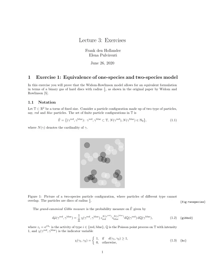
(1.1) where N(γ) denotes the cardinality of γ. Figure 1: Picture of a two-species particle configuration, where particles of different type cannot

• verlap. The particles are discs of radius 1

2.

{fig:twospecies}

The grand-canonical Gibbs measure is the probability measure on ˜ Γ given by d˜ µ(γred, γblue) = 1 ˜ Ξ χ(γred, γblue) zN(γred)

red

zN(γblue)

blue

dQ(γred) dQ(γblue), (1.2)

{gibbs2}

where zi = eβλi is the activity of type i ∈ {red, blue}, Q is the Poisson point process on T with intensity 1, and χ(γred, γblue) is the indicator variable χ(γ1, γ2) =

• 1,

if d(γ1, γ2) ≥ 1, 0,

• therwise,

(1.3)

{hc}

1

where d(γ1, γ2) means the minimal distance between points in the sets γ1 and γ2. Particles can be viewed as discs of radius 1

2 (as in Fig. 1). The indicator χ(γred, γblue) means that discs of the same

type can overlap while discs of different type cannot overlap. The normalising partition function is ˜ Ξ =

• ˜

Γ

χ(γred, γblue) zN(γred)

red

zN(γblue)

blue

dQ(γred) dQ(γblue). (1.4)

1.2 Exercise

Fix zred, zblue > 0. Let πblue : ˜ Γ → Γ be the projection that maps (γred, γblue) to γblue. Define β, z by putting (zred, zblue) = (β, z eβπ), (1.5)

{chov}

and let µ = µβ,z be the associated one-species Gibbs measure, i.e. dµ(γ) = 1 Ξ zN(γ) e−βH(γ)dQ(γ). (1.6) (see slides of Lecture 3 for the notation of the one-species WR-model). Prove that ˜ µ ◦ π−1

blue = µ

(1.7)

{duality}

1.3 Guidelines for solving the exercise

• Step 1: Fix the centers of the blue discs and integrate over the centers of the red discs. Prove

that 1 ˜ Ξ

• Γ

Q(dγred) zN(γred)

red

zN(γblue)

blue

χ(γred, γblue) = 1 ˜ Ξ e(β−1)|T| z eβπN(γblue) e−βV (γblue), (1.8) where V (γ) is the volume of the halo h(γ) of γ. [Hint: Use that the union of the blue discs is impenetrable for the red discs, so that the halo of the blue discs is a “forbidden area” for the centres of the red discs.]

• Step 2: Explain why

1 Ξ = e(β−1)|T| ˜ Ξ (1.9) and use this to conclude the proof.

2 Exercise 2: LDP for the Widom-Rowlinson model

In this exercise you will prove a Large Deviation Principle (LDP) for the equilibrium measure µβ of the WR-model, as shown in den Hollander, Jansen, Koteck´ y and Pulvirenti [2].

2.1 Notation and LDP setting

To make the exercise self contained, we recall the definition of the Large Deviation Principle (see e.g. den Hollander [1, Chapter 3]).

{defldp}

Definition 2.1. A sequence of probability measures (Pn)n∈N on a Polish space X is said to satisfy the large deviation principle (LDP) with rate n and with rate function I : X → [0, ∞] if

• I has compact level sets and I ≡ ∞,
• lim infn→∞ 1

n log Pn(O) ≥ −I(O), for all O ⊂ X open,

2

• lim supn→∞

1 n log Pn(C) ≤ −I(C), for all C ⊂ X closed,

where I(A) = infx∈A I(x). Informally, the LDP says that if Bδ(x) is the open ball of radius δ > 0 centred at x ∈ X, then Pn(Bδ(x)) = e−[1+o(1)] n I(x) (2.1) when n → ∞ followed by δ ↓ 0. We also recall the following version of Varadhan’s lemma (see e.g. den Hollander [1, Theorem 3.17]).

{varadhan}

Theorem 2.2 (Tilted LDP). Let (Pn)n∈N satisfy the LDP on X with rate n and rate function I. Let F ∈ Cb(X), the space of bounded continuous functions on X. Define Jn(S) =

• S

enF (x)Pn(dx), S ⊂ X Borel. (2.2) Then (P F

n )n∈N defined by

P F

n (S) = Jn(S)

Jn(X), S ⊂ X Borel, (2.3) satisfies the LDP on X with rate n and rate function IF (x) = sup

y∈X

[F(y) − I(y)] − [F(x) − I(x)] . (2.4) Let F be the family of non-empty closed (and hence compact) subsets of the torus T. By equipping F with the Hausdorff metric, we turn it into a compact metric space. The halo of any F ∈ F is given by the Minkowski addition, i.e., F + = F + B(0) =

• x∈B(0)

(F + x) = h(F), (2.5)

{F+def}

where B(0) is the ball of radius 1 centered at x = 0. Now recall the formula for the equilibrium Gibbs measure of the WR-model at inverse temperature β and activity z = κzc(β) = κβe−βπ given on the slides, µβ(dγ) = 1 Ξ (κβ)N(γ) e−βV (γ) Q(dγ), γ ∈ Γ, (2.6)

{gibbs1alt}

where V (γ) = |h(γ)| and Ξ is the normalising partition function. This is a probability measure on the space Γ ⊂ F of particle configurations. We identify µβ on Γ with the measure on F supported on Γ.

2.2 Exercise

Prove that the family of probability measures (µβ)β≥1 on F, supported on Γ ⊂ F, satisfies the LDP with rate β and rate function IWR given by IWR = JWR − inf

F JWR,

JWR(F) = |F +| − κ|F|, F ∈ F. (2.7)

{ratef}

2.3 Guidelines for solving the exercise

• Step 1: Let Πκβ be the homogeneous Poisson point process on T with intensity κβ. Denote its

law by Pκβ. Show that µβ is absolutely continuous with respect to Pκβ, with Radon-Nikodym derivative dµβ dPκβ (γ) = exp(−β|h(γ)|)

• Γ exp(−β|h|) dPκβ

, γ ∈ Γ. (2.8) 3

• Step 2: Use the following fact (Schreiber [3], [4, Theorem 1]): the family (Pκβ)β≥1 satisfies the

LDP with rate β and with rate function I(F) = κ|T \ F|, F ∈ F. Note that, by the properties of the Poisson point process, P(Πκβ ⊂ F) = P(Πκβ ∩ (T \ F) = ∅) = e−βI(F ), F ∈ F.

• Step 3: Now apply Theorem 2.2 to the family (µβ)β≥1, where µβ(C) = Jβ(C)/Jβ(Γ), ∀ C ⊂ F

Borel, with Jβ(C) =

• C

exp(−β|h(γ)|) dPκβ(γ). (2.9) [Hint: Use that the map F → |F +| = |h(F)| is continuous with respect to the Hausdorff metric.]

3 Exercise 3: LDP for the halo shape and the halo volume

In this exercise you will see how to obtain the leading order term of the average metastable crossover time via two Large Deviation Principles and an isoperimetric inequality, as shown in den Hollander, Jansen, Koteck´ y and Pulvirenti [2]. Even though this exercise uses the outcome of Exercise 2, you may try to solve it even when you did not manage to solve Exercise 2.

3.1 Notation and useful results

Let S ⊂ F be the collection of all sets that are admissible, i.e., S = {S ⊂ T: ∃ F such that h(F) = S}. (3.1)

{adm}

There is a unique maximal F such that h(F) = S, which we denote by S− and which equals S− = {x ∈ S : B(x) ⊂ S}. We can view the halo h(γ) as a random variable taking values in the space S, endowed with the Hausdorff distance. We recall the following corner stone from large deviation theory (see e.g. den Hollander [1, Theorem 3.20]).

{contraction}

Theorem 3.1 (Contraction principle). Let (Pn)n∈N satisfy the LDP on X with rate n and with rate function I. Let Y be a second Polish space, and T : X → Y a continuous map. Then (Qn)n∈N on Y defined by Qn = Pn ◦ T −1 satisfies the LDP on Y with rate n and with rate function J given by J (y) = inf

x∈X : T (x)=y I(x).

(3.2) Finally, for completeness we write down the following result that you have seen in Lecture 3 (see also den Hollander, Jansen, Koteck´ y and Pulvirenti [2, Theorem 2.2]).

{thm:isope}

Theorem 3.2 (Minimisers of rate function for halo volume). For every R ∈ (1, L

π + 1 2),

min

• |S| − κ|S−|: S ∈ S, |S| = πR2

= πR2 − κπ(R − 1)2, (3.3)

{isope}

and the minimisers are the discs of radius R. (We refer to [2] for a statement about the stability of the minimisers under small perturbations. Since this statement is not needed for the exercise, we omitted it.)

3.2 Exercise

(i) Prove that the family of probability measures (µβ(h(γ) ∈ · ))β≥1 satisfies the LDP on S with rate β and rate function I given by I(S) = |S| − κ|S−| − (1 − κ)|T|, S ∈ S. (3.4) 4

(ii) Prove that the family of probability measures (µβ(V (γ) ∈ · ))β≥1 satisfies the LDP on [0, ∞) with rate β and with rate function I∗ given by I∗(A) = inf{I(S): S ∈ S, |S| = A}. (3.5)

{eq:ivol}

(iii) Explain the following (informal) statement, for β → ∞, µβ(V (γ) ≈ πR2) ≈ exp

• −β
• πR2 − κπ(R − 1)2

+ (1 − κ)β|T|

• .

(3.6)

{asym}

3.3 Guidelines for solving the exercise

• Step 1: Use the contraction principle, i.e., Theorem 3.1, and Exercise 2, i.e., (2.7), to prove that

the family (µβ(h(γ) ∈ · ))β≥1 satisfies the LDP with rate β and with rate function I = J − inf

F J,

J(S) = inf

• |F +| − κ|F|: F ∈ F, F + = S
• ,

S ∈ S. (3.7) [Hint: Use that the map F → S defined by F → S = F + is continuous with respect to the Hausdorff metric.]

• Step 2: Show that J(S) = |S| − κ|S−| via upper and lower bounds.

[Hint: Use that if F + = S, then F ⊂ S−. If F = S−, then for S to be an admissible set it must be that F + = (S−)+ = S.]

• Step 3: Use again the contraction principle, i.e., Theorem 3.1, and the previous steps, to prove

that the family (µβ(V (γ) ∈ · ))β≥1 satisfies the LDP with rate β and with rate function I∗ given by the difference of two infima. [Hint: Use that the map F → |F +| = |h(F)| is continuous.]

• Step 4: Compute the two infima in I∗. First set A = πR2 and use Theorem 3.2. Afterwards

show that infS J = (1 − κ)|T| because κ ∈ (1, ∞). Conclude by explaining in words what the asymptotic expression (3.6) means.

References

[1] F. den Hollander, Large Deviations, Fields Institute Monographs 14, American Mathematical Society, Providence RI, 2000. [2] F. den Hollander, S. Jansen, R. Koteck´ y and E. Pulvirenti, The Widom-Rowlinson model: Meso- scopic fluctuations for the critical droplet, preprint 2019 [arXiv:1907.00453]. [3] T. Schreiber, Large deviation principle for set-valued union processes, Prob. Math. Statist. 20 (2000) 273–285. [4] T. Schreiber, Asymptotic geometry of high-density smooth-grained Boolean models in bounded domains, Adv. Appl. Prob. (SGSA) 35 (2003) 913–936. [5] B. Widom and J.S. Rowlinson, New model for the study of liquid-vapor phase transitions, J.

• Chem. Phys. 52 (1970) 1670–1684.

5