Lecture 18: Greedy Algorithms + Midterm Review Tim LaRock - PowerPoint PPT Presentation
Lecture 18: Greedy Algorithms + Midterm Review Tim LaRock larock.t@northeastern.edu bit.ly/cs3000syllabus Business Homework 5 due tonight at midnight Boston time, solutions will be released tomorrow morning No class tomorrow, midterm review
Lecture 18: Greedy Algorithms + Midterm Review Tim LaRock larock.t@northeastern.edu bit.ly/cs3000syllabus
Business Homework 5 due tonight at midnight Boston time, solutions will be released tomorrow morning No class tomorrow, midterm review moved to today Extra credit assignment available as of yesterday • Optional • 6 points on the final exam • Available until Sunday June 21 st Midterm 2 to be released tomorrow night, due Friday night • Topics: Graph algorithms and network flow
Greedy Algorithms • For some problems, we can think of simple decision making rules that intuitively guide us towards a solution • Best-first search: We want to find shortest paths/minimum trees, so only choose edges that can be included in these solutions! • Applying this idea does not always work as intended! • Maximum flow: We tried assigning flow based on best-first search, but we showed that the algorithm will get stuck if it is not able to modify the flow! • Algorithms that rely on repeatedly making optimal local decisions to eventually reach an optimal global solution are called greedy algorithms
Example: Files on Tape Before any of us were born, computers used to exist on magnetic tape. Imagine we have such a tape, split in to segments we will call “blocks”, where each block contains data from a single file. Each file is referred to by an integer index 𝑗 , and has length in blocks 𝑀[𝑗] . 1 1 1 2 2 3 3 3 4 4 To read file 𝑙 , the tape head needs to first skip all of the files before 𝑙 . Therefore, the cost of accessing file 𝑙 can be written as , 𝑑𝑝𝑡𝑢 𝑙 = + 𝑀[𝑗] -./
Example: Files on Tape 1 1 1 2 2 3 3 3 4 4 Assuming all files are equally likely to be accessed, we can write the expected (equivalently, average) cost of accessing file k as 5 5 , 𝔽 𝑑𝑝𝑡𝑢 = 1 = 1 𝑜 + 𝑑𝑝𝑡𝑢(𝑗) 𝑜 + + 𝑀[𝑗] -./ ,./ -./
𝔽 𝑑𝑝𝑡𝑢 = 1 4 ⋅ 𝑑𝑝𝑡𝑢(1) + 𝑑𝑝𝑡𝑢(2) + 𝑑𝑝𝑡𝑢(3) + 𝑑𝑝𝑡𝑢(4) Example: Files on Tape = 1 4 ⋅ 3 + 5 + 8 + 10 = 26 4 1 1 1 2 2 3 3 3 4 4 Assuming all files are equally likely to be accessed, we can write the expected (equivalently, average) cost of accessing file k as 5 5 , 𝔽 𝑑𝑝𝑡𝑢 = 1 = 1 𝑜 + 𝑑𝑝𝑡𝑢(𝑗) 𝑜 + + 𝑀[𝑗] -./ ,./ -./
What order should we keep the files in? 𝔽 𝑑𝑝𝑡𝑢 = 26 1 1 1 2 2 3 3 3 4 4 4 We can modify the order of the files on the tape, resulting in a permutation 𝜌 where 𝜌(𝑗) returns the index of the file in the 𝑗 th block. We can then rewrite the expected (average) cost of accessing file k as 5 , 𝔽 𝑑𝑝𝑡𝑢(𝜌) = 1 𝑜 + + 𝑀[𝜌(𝑗)] ,./ -./ Intuitively: To minimize average cost, we should store the smallest files first, otherwise we will need to unnecessarily spend time skipping the large files to read smaller ones! 2 2 4 4 1 1 1 3 3 3 But how do we prove that this is the optimal strategy?
What order should we keep the files in? 𝔽 𝑑𝑝𝑡𝑢 = 26 1 1 1 2 2 3 3 3 4 4 4 We can modify the order of the files on the tape, resulting in a permutation 𝜌 where 𝜌(𝑗) returns the index of the file in the 𝑗 th block. We can then rewrite the expected (average) cost of accessing file k as 5 , 𝔽 𝑑𝑝𝑡𝑢(𝜌) = 1 𝑜 + + 𝑀[𝜌(𝑗)] ,./ -./ Intuitively: To minimize average cost, we should store the smallest files first, otherwise we will need to unnecessarily spend time skipping the large files to read smaller ones! 2 2 4 4 1 1 1 3 3 3 But how do we prove that this is the optimal strategy? 𝔽 𝑑𝑝𝑡𝑢(𝜌) = 2 + 4 + 7 + 10 = 23 4 4
Greedy Algorithm for Storing Files Input: A set of files labeled 1 … 𝑜 with lengths 𝑀[𝑗] Output: An ordering of the files on the tape Repeat until all files are on the tape: 1. Find the unwritten file with minimum length (break ties arbitrarily) 2. Write that file to the tape
Greedy Algorithm for Storing Files Input: A set of files labeled 1 … 𝑜 with lengths 𝑀[𝑗] Output: An ordering of the files on the tape Repeat until all files are on the tape: 1. Find the unwritten file with minimum length (break ties arbitrarily) 2. Write that file to the tape How can we show this is optimal?
Proof of optimality 1 1 1 2 2 3 3 3 4 4 Claim: 𝔽 𝑑𝑝𝑡𝑢 𝜌 is minimized when 𝑀 𝜌 𝑗 ≤ 𝑀[𝜌 𝑗 + 1 ] for all 𝑗 . Proof: Let a = 𝜌 𝑗 and 𝑐 = 𝜌(𝑗 + 1) and suppose 𝑀 𝑏 > 𝑀[𝑐] for some index 𝑗 . If we swap the files 𝑏 and 𝑐 on the tape, then the cost of accessing 𝑏 increases by 𝑀[𝑐] and the cost of accessing 𝑐 decreases by 𝑀[𝑏] . H I JH[K] Overall, the swap changes the expected cost by . 5 This change represents an improvement because 𝑀 𝑐 < 𝑀[𝑏] . Thus, if the files are out of order, we can decrease expected cost by swapping pairs to put them in order.
Proof of optimality 1 1 1 2 2 3 3 3 4 4 Claim: 𝔽 𝑑𝑝𝑡𝑢 𝜌 is minimized when 𝑀 𝜌 𝑗 ≤ 𝑀[𝜌 𝑗 + 1 ] for all 𝑗 . Proof: Let a = 𝜌 𝑗 and 𝑐 = 𝜌(𝑗 + 1) and suppose 𝑀 𝑏 > 𝑀[𝑐] for some index 𝑗 . If we swap the files 𝑏 and 𝑐 on the tape, then the cost of accessing 𝑏 increases by 𝑀[𝑐] and the cost of accessing 𝑐 decreases by 𝑀[𝑏] . H I JH[K] Overall, the swap changes the expected cost by . 5 This change represents an improvement because 𝑀 𝑐 < 𝑀[𝑏] . Thus, if the files are out of order, we can decrease expected cost by swapping pairs to put them in order.
Proof of optimality 1 1 1 2 2 3 3 3 4 4 Claim: 𝔽 𝑑𝑝𝑡𝑢 𝜌 is minimized when 𝑀 𝜌 𝑗 ≤ 𝑀[𝜌 𝑗 + 1 ] for all 𝑗 . Proof: Let a = 𝜌 𝑗 and 𝑐 = 𝜌(𝑗 + 1) and suppose 𝑀 𝑏 > 𝑀[𝑐] for some index 𝑗 . If we swap the files 𝑏 and 𝑐 on the tape, then the cost of accessing 𝑏 increases by 𝑀[𝑐] and the cost of accessing 𝑐 decreases by 𝑀[𝑏] . H I JH[K] Overall, the swap changes the expected cost by . 5 This change represents an improvement because 𝑀 𝑐 < 𝑀[𝑏] . Thus, if the files are out of order, we can decrease expected cost by swapping pairs to put them in order.
Proof of optimality 1 1 1 2 2 3 3 3 4 4 Claim: 𝔽 𝑑𝑝𝑡𝑢 𝜌 is minimized when 𝑀 𝜌 𝑗 ≤ 𝑀[𝜌 𝑗 + 1 ] for all 𝑗 . Proof: Let a = 𝜌 𝑗 and 𝑐 = 𝜌(𝑗 + 1) and suppose 𝑀 𝑏 > 𝑀[𝑐] for some index 𝑗 . If we swap the files 𝑏 and 𝑐 on the tape, then the cost of accessing 𝑏 increases by 𝑀[𝑐] and the cost of accessing 𝑐 decreases by 𝑀[𝑏] . H K JH[I] Overall, the swap changes the expected cost by . 5 This change represents an improvement because 𝑀 𝑐 < 𝑀[𝑏] . Thus, if the files are out of order, we can decrease expected cost by swapping pairs to put them in order.
Proof of optimality 1 1 1 2 2 3 3 3 4 4 Claim: 𝔽 𝑑𝑝𝑡𝑢 𝜌 is minimized when 𝑀 𝜌 𝑗 ≤ 𝑀[𝜌 𝑗 + 1 ] for all 𝑗 . Proof: Let a = 𝜌 𝑗 and 𝑐 = 𝜌(𝑗 + 1) and suppose 𝑀 𝑏 > 𝑀[𝑐] for some index 𝑗 . If we swap the files 𝑏 and 𝑐 on the tape, then the cost of accessing 𝑏 increases by 𝑀[𝑐] and the cost of accessing 𝑐 decreases by 𝑀[𝑏] . H K JH[I] Overall, the swap changes the expected cost by . 5 This change represents an improvement because 𝑀 𝑐 < 𝑀[𝑏] . Thus, if the files are out of order, we can decrease expected cost by swapping pairs to put them in order.
Proof of optimality 1 1 1 2 2 3 3 3 4 4 Claim: 𝔽 𝑑𝑝𝑡𝑢 𝜌 is minimized when 𝑀 𝜌 𝑗 ≤ 𝑀[𝜌 𝑗 + 1 ] for all 𝑗 . Proof: Let a = 𝜌 𝑗 and 𝑐 = 𝜌(𝑗 + 1) and suppose 𝑀 𝑏 > 𝑀[𝑐] for some index 𝑗 . If we swap the files 𝑏 and 𝑐 on the tape, then the cost of accessing 𝑏 increases by 𝑀[𝑐] and the cost of accessing 𝑐 decreases by 𝑀[𝑏] . H K JH[I] Overall, the swap changes the expected cost by . 5 This change represents an improvement because 𝑀 𝑐 < 𝑀[𝑏] . MN Average cost for example above: Thus, if the files are out of order, we can decrease expected cost by swapping pairs to put O / MP Average cost after swapping files 1 and 2: O 2 + 5 + 8 + 10 = them in order. O 26 4 + 2 − 3 = 26 − 1 = 25 4 4 4
Proof of optimality 1 1 1 2 2 3 3 3 4 4 Claim: 𝔽 𝑑𝑝𝑡𝑢 𝜌 is minimized when 𝑀 𝜌 𝑗 ≤ 𝑀[𝜌 𝑗 + 1 ] for all 𝑗 . Proof: Let a = 𝜌 𝑗 and 𝑐 = 𝜌(𝑗 + 1) and suppose 𝑀 𝑏 > 𝑀[𝑐] for some index 𝑗 . If we swap the files 𝑏 and 𝑐 on the tape, then the cost of accessing 𝑏 increases by 𝑀[𝑐] and the cost of accessing 𝑐 decreases by 𝑀[𝑏] . H K JH[I] Overall, the swap changes the expected cost by . 5 This change represents an improvement because 𝑀 𝑐 < 𝑀[𝑏] . Thus, if the files are out of length-order, we can decrease expected cost by swapping pairs to put them in order.
Wrap-up Greedy algorithms repeatedly apply a simple rule to eventually find an optimal solution Inductive Exchange Arguments are strategies for proving correctness of some greedy algorithms Next Week: Data Compression with Huffman Codes Proof strategies for greedy algorithms Inductive exchange Greedy-stays-ahead
Midterm 2 Review/Q&A
Recommend
More recommend
Explore More Topics
Stay informed with curated content and fresh updates.
