Lecture 15: Software Quality Assurance 2015-07-09 Prof. Dr. Andreas - - PDF document

SLIDE 1

– 15 – 2015-07-09 – main –

Softwaretechnik / Software-Engineering

Lecture 15: Software Quality Assurance

2015-07-09

• Prof. Dr. Andreas Podelski, Dr. Bernd Westphal

Albert-Ludwigs-Universit¨ at Freiburg, Germany

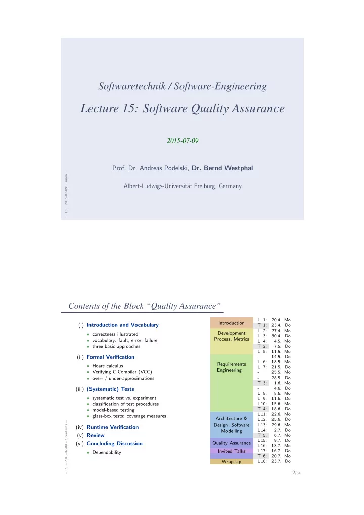
Contents of the Block “Quality Assurance”

– 15 – 2015-07-09 – Scontents –

2/54 (i) Introduction and Vocabulary

• correctness illustrated
• vocabulary: fault, error, failure
• three basic approaches

(ii) Formal Verification

• Hoare calculus
• Verifying C Compiler (VCC)
• over- / under-approximations

(iii) (Systematic) Tests

• systematic test vs. experiment
• classification of test procedures
• model-based testing
• glass-box tests: coverage measures

(iv) Runtime Verification (v) Review (vi) Concluding Discussion

• Dependability

L 1: 20.4., Mo

Introduction

T 1: 23.4., Do L 2: 27.4., Mo L 3: 30.4., Do L 4: 4.5., Mo

Development Process, Metrics

T 2: 7.5., Do L 5: 11.5., Mo

• 14.5., Do

L 6: 18.5., Mo L 7: 21.5., Do

• 25.5., Mo
• 28.5., Do

Requirements Engineering

T 3: 1.6., Mo

• 4.6., Do

L 8: 8.6., Mo L 9: 11.6., Do L 10: 15.6., Mo T 4: 18.6., Do L 11: 22.6., Mo L 12: 25.6., Do L 13: 29.6., Mo L 14: 2.7., Do

Architecture & Design, Software Modelling

T 5: 6.7., Mo L 15: 9.7., Do

Quality Assurance

L 16: 13.7., Mo

Invited Talks

L 17: 16.7., Do T 6: 20.7., Mo

Wrap-Up

L 18: 23.7., Do

SLIDE 2

Contents & Goals

– 15 – 2015-07-09 – Sprelim –

3/54

Last Lecture:

• Completed the block “Architecture & Design”

This Lecture:

• Educational Objectives: Capabilities for following tasks/questions.
• When do we call a software correct?
• What is fault, error, failure? How are they related?
• What is formal and partial correctness?
• What is a Hoare triple (or correctness formula)?
• Is this program (partially) correct?
• Prove the (partial) correctness of this WHILE-program using PD.
• What can we conclude from the outcome of tools like VCC?
• Content:
• Introduction, Vocabulary
• WHILE-program semantics, partial & total correctness
• Correctness proofs with the calculus PD.
• The Verifying C Compiler (VCC)

Introduction

– 15 – 2015-07-09 – main –

4/54

SLIDE 3

SLIDE 4

SLIDE 5

Back To Lecture No. 1

– 15 – 2015-07-09 – Svintro –

7/54

• Definition. A software specification is a finite description S of a (possibly

infinite) set S of softwares, i.e. S = {(S1, · 1), . . . }. The (possibly partial) function · : S → S is called interpretation of S .

We define: Software S is correct wrt. software specification S if and only if (S, · ) ∈ S .

• Note: no specification, no correctness. Without specification, S is neither correct

nor not correct — it’s just some software then.

SLIDE 6

Vocabulary

– 15 – 2015-07-09 – Svintro –

9/54

software quality assurance — See: quality assurance.

IEEE 610.12 (1990)

quality assurance — (1) A planned and systematic pattern of all actions necessary to provide adequate confidence that an item or product conforms to established technical requirements. (2) A set of activities designed to evaluate the process by which products are developed or manufactured.

IEEE 610.12 (1990)

Note: in order to trust a product, it can be built well, or proven to be good (at best: both) — both is QA in the sense of (1).

Concepts of Software Quality Assurance

– 15 – 2015-07-09 – Svintro –

10/54 software quality assurance

project management

• rganisational

software examination

analytic

examination by humans

non-mech.

inspection review manual proof

• comp. aided

human exam.

semi-mech.

e.g. interactive prover examination with computer

mechanical

static checking

analyse

check against rules consistency checks quantitative examina- tion dynamic checking (test)

execute

formal verification

prove

constructive software engineering

constructive

e.g. code generation (Ludewig and Lichter, 2013)

SLIDE 7

Fault, Error, Failure

– 15 – 2015-07-09 – Svintro –

11/54 fault — abnormal condition that can cause an element or an item to fail.

Note: Permanent, intermittent and transient faults (especially soft-errors) are considered. Note: An intermittent fault occurs time and time again, then disappears. This type of fault can occur when a component is on the verge of breaking down or, for example, due to a glitch in a switch. Some systematic faults (e.g. timing marginalities) could lead to intermittent faults. ISO 26262 (2011)

error — discrepancy between a computed, observed or measured value or condition, and the true, specified, or theoretically correct value or condition.

Note: An error can arise as a result of unforeseen operating conditions or due to a fault within the system, subsystem or, component being considered. Note: A fault can manifest itself as an error within the considered element and the error can ultimately cause a failure. ISO 26262 (2011)

failure — termination of the ability of an element, to perform a function as required.

Note: Incorrect specification is a source of failure. ISO 26262 (2011)

We want to avoid failures, thus we try to detect faults, e.g. by looking for errors.

SLIDE 8

So, What Do We Do?

– 15 – 2015-07-09 – Svintro –

13/54

LSC: buy water AC: true AM: invariant I: strict User CoinValidator ChoicePanel Dispenser C50 p W A T E R ¬(C50! ∨ E1! ∨ pSOFT! ∨ pTEA! ∨ pFILLUP! water in stock dWATER OK ¬(dSoft! ∨ dTEA!)

• If we are lucky, the requirement specification

is a constraint on computation paths.

• LSC ‘buy water’ is such a software specification S .
• It denotes all controller softwares which “faithfully” sell water.

(Or which refuse to accept C50 coins, or block the ‘WATER’ button).

• Formally

buy waterspec = {S | S satisfies ‘buy water’}.

• In pictures:

(Σ × A)ω

all computation paths satisfying ‘buy water’ S of one acceptable software S

(Σ × A)ω

S of one not acceptable software S

• Then we can check correctness of a given software S

by examining its computation paths S.

Three Basic Directions

– 15 – 2015-07-09 – Svintro –

14/54

(Σ × A)ω

all computation paths satisfying specification

SLIDE 9

Formal Verification

– 15 – 2015-07-09 – main –

15/54

SLIDE 10

Correctness Formulae (“Hoare Triples”)

– 15 – 2015-07-09 – Spsq –

16/54

• One style of requirements specifications: pre- and post-conditions

(on whole programs or on procedures).

• Let S be a program with states from Σ and let p and q be formulae

such that there is a satisfaction relation | = ⊆ Σ × {p, q}.

• S is called partially correct wrt. p and q, denoted by |

= {p} S {q}, if and only if ∀ π = σ0

α1

− → σ1

α2

− → σ2 · · · σn−1

αn

− − → σn ∈ S • σ0 | = p = ⇒ σn | = q

(“if S terminates from a state satisfying p, then the final state of that computation satisfies q”)

• S is called totally correct wrt. p and q, denoted by |

=tot {p} S {q}, if and only if

• {p} S {q} (S is partially correct), and
• ∀ π ∈ S • π0 |

= p = ⇒ |π| ∈ N0 (S terminates from all states satisfying p; length of paths: | · | : Π → N0 ˙ ∪ {⊥}).

Example

– 15 – 2015-07-09 – Spsq –

17/54

Computing squares (of numbers 0, . . . , 27).

• Pre-condition: p ≡ 0 ≤ x ≤ 27, post-condition: q ≡ y = x2.
• Program S1:

1

i nt y = x ;

2

y = ( x − 1) ∗ x + y ;

| =? {p} S1 {q}, | =?

tot {p} S1 {q}

• Program S2:

1

i nt y = x ;

2

i nt z ; // u n i n i t i a l i s e d

3

y = (( x − 1) ∗ x + y ) + z ;

| =? {p} S2 {q}, | =?

tot {p} S2 {q}

• Program S3:

1

i nt y = x ;

2

y = ( x − 1) ∗ x + y ;

3

while ( 1 ) ;

| =? {p} S3 {q}, | =?

tot {p} S3 {q}

• Program S4:

1

i nt y = x ;

2

i nt z ; // u n i n i t i a l i s e d

3

y = (( x − 1) ∗ x + y ) + z ;

4

while ( z ) ;

| =? {p} S4 {q}, | =?

tot {p} S4 {q}

SLIDE 11

Deterministic Programs

– 15 – 2015-07-09 – Spsq –

18/54

Syntax: S := skip | u := t | S1; S2 | if B then S1 else S2 fi | while B do S1 do where u is a variable, t a type-compatible expression, B a Boolean expression. Semantics: (is induced by the following transition relation)

(i) skip, σ → E, σ (ii) u := t, σ → E, σ[u := σ(t)] (iii) S1, σ → S2, τ S1; S, σ → S2; S, τ (iv) if B then S1 else S2 fi, σ → S1, σ, if σ | = B, (v) if B then S1 else S2 fi, σ → S2, σ, if σ | = B, (vi) while B do S do, σ → S; while B do S do, σ, if σ | = B, (vii) while B do S do, σ → E, σ, if σ | = B, E denotes the empty program; define E; S ≡ S; E ≡ S. Note: the first component of S, σ is a program (structural operational semantics).

Computations of Deterministic Programs

– 15 – 2015-07-09 – Spsq –

19/54 Definition. (i) A transition sequence of S (starting in σ) is a finite or infinite sequence S, σ = S0, σ0 → S1, σ1 → . . .

(that is, Si, σi and Si+1, σi+1 are in transition relation for all i).

(ii) A computation (path) of S (starting in σ) is a maximal transition se- quence of S (starting in σ), i.e. infinite or not extendible. (iii) A computation of S is said to a) terminate in τ if and only if it is finite and ends with E, τ, b) diverge if and only if it is infinite. S can diverge from σ if and only if there is a diverging computation starting in σ. (iv) We use →∗ to denote the transitive, reflexive closure of →.

• Lemma. For each deterministic program S and each state σ,

there is exactly one computation of S which starts in σ.

SLIDE 12

Example

– 15 – 2015-07-09 – Spsq –

20/54

(i) skip, σ → E, σ E; S ≡ S; E ≡ S (ii) u := t, σ → E, σ[u := σ(t)] (iii) S1, σ → S2, τ S1; S, σ → S2; S, τ (iv) if B then S1 else S2 fi, σ → S1, σ, if σ | = B, (v) if B then S1 else S2 fi, σ → S2, σ, if σ | = B, (vi) while B do S do, σ → S; while B do S do, σ, if σ | = B, (vii) while B do S do, σ → E, σ, if σ | = B,

Consider program S ≡ a[0] := 1; a[1] := 0; while a[x] = 0 do x := x + 1 do and a state σ with σ | = x = 0.

Example

– 15 – 2015-07-09 – Spsq –

20/54

(i) skip, σ → E, σ E; S ≡ S; E ≡ S (ii) u := t, σ → E, σ[u := σ(t)] (iii) S1, σ → S2, τ S1; S, σ → S2; S, τ (iv) if B then S1 else S2 fi, σ → S1, σ, if σ | = B, (v) if B then S1 else S2 fi, σ → S2, σ, if σ | = B, (vi) while B do S do, σ → S; while B do S do, σ, if σ | = B, (vii) while B do S do, σ → E, σ, if σ | = B,

Consider program S ≡ a[0] := 1; a[1] := 0; while a[x] = 0 do x := x + 1 do and a state σ with σ | = x = 0. S, σ

SLIDE 13

Example

– 15 – 2015-07-09 – Spsq –

20/54

(i) skip, σ → E, σ E; S ≡ S; E ≡ S (ii) u := t, σ → E, σ[u := σ(t)] (iii) S1, σ → S2, τ S1; S, σ → S2; S, τ (iv) if B then S1 else S2 fi, σ → S1, σ, if σ | = B, (v) if B then S1 else S2 fi, σ → S2, σ, if σ | = B, (vi) while B do S do, σ → S; while B do S do, σ, if σ | = B, (vii) while B do S do, σ → E, σ, if σ | = B,

Consider program S ≡ a[0] := 1; a[1] := 0; while a[x] = 0 do x := x + 1 do and a state σ with σ | = x = 0. S, σ

(ii),(iii)

− − − − − → a[1] := 0; while a[x] = 0 do x := x + 1 do, σ[a[0] := 1]

Example

– 15 – 2015-07-09 – Spsq –

20/54

(i) skip, σ → E, σ E; S ≡ S; E ≡ S (ii) u := t, σ → E, σ[u := σ(t)] (iii) S1, σ → S2, τ S1; S, σ → S2; S, τ (iv) if B then S1 else S2 fi, σ → S1, σ, if σ | = B, (v) if B then S1 else S2 fi, σ → S2, σ, if σ | = B, (vi) while B do S do, σ → S; while B do S do, σ, if σ | = B, (vii) while B do S do, σ → E, σ, if σ | = B,

Consider program S ≡ a[0] := 1; a[1] := 0; while a[x] = 0 do x := x + 1 do and a state σ with σ | = x = 0. S, σ

(ii),(iii)

− − − − − → a[1] := 0; while a[x] = 0 do x := x + 1 do, σ[a[0] := 1]

(ii),(iii)

− − − − − → while a[x] = 0 do x := x + 1 do, σ′

(vi)

− − → x := x + 1; while a[x] = 0 do x := x + 1 do, σ′ where σ′ = σ[a[0] := 1][a[1] := 0].

SLIDE 14

Example

– 15 – 2015-07-09 – Spsq –

20/54

(i) skip, σ → E, σ E; S ≡ S; E ≡ S (ii) u := t, σ → E, σ[u := σ(t)] (iii) S1, σ → S2, τ S1; S, σ → S2; S, τ (iv) if B then S1 else S2 fi, σ → S1, σ, if σ | = B, (v) if B then S1 else S2 fi, σ → S2, σ, if σ | = B, (vi) while B do S do, σ → S; while B do S do, σ, if σ | = B, (vii) while B do S do, σ → E, σ, if σ | = B,

Consider program S ≡ a[0] := 1; a[1] := 0; while a[x] = 0 do x := x + 1 do and a state σ with σ | = x = 0. S, σ

(ii),(iii)

− − − − − → a[1] := 0; while a[x] = 0 do x := x + 1 do, σ[a[0] := 1]

(ii),(iii)

− − − − − → while a[x] = 0 do x := x + 1 do, σ′

(vi)

− − → x := x + 1; while a[x] = 0 do x := x + 1 do, σ′

(ii),(iii)

− − − − − → while a[x] = 0 do x := x + 1 do, σ′[x := 1]

(vii)

− − − → E, σ′[x := 1] where σ′ = σ[a[0] := 1][a[1] := 0].

Input/Output Semantics of Deterministic Programs

– 15 – 2015-07-09 – Spsq –

21/54

Definition. Let S be a deterministic program. (i) The semantics of partial correctness is the function MS : Σ → 2Σ with MS(σ) = {τ | S, σ →∗ E, τ}. (ii) The semantics of total correctness is the function MtotS : Σ → 2Σ ˙ ∪ {⊥} with MtotS(σ) = MS(σ) ∪ {⊥ | S can diverge from σ}. ⊥ is an error state representing divergence. Note: MtotS(σ) has exactly one element, MS(σ) at most one.

SLIDE 15

Correctness of Deterministic Programs

– 15 – 2015-07-09 – Spsq –

22/54

Definition. (i) A correctness formula {p} S {q} holds in the sense of partial correctness, denoted by | = {p} S {q}, if and only if MS(p) ⊆ q. We say S is partially correct wrt. p and q. (ii) A correctness formula {p} S {q} holds in the sense of total cor- rectness, denoted by | =tot {p} S {q}, if and only if MtotS(p) ⊆ q. We say S is totally correct wrt. p and q.

Example: Correctness

– 15 – 2015-07-09 – Spsq –

23/54

• By the previous example, we have shown

| = {x = 0} S {x = 1} and | =tot {x = 0} S {x = 1}.

(because we only assumed σ | = x = 0 for the example, which is exactly the precondition.)

• We have also shown:

| = {x = 0} S {x = 1 ∧ a[x] = 0}.

• The following correctness formula does not hold for S:

{x = 2} S {true}.

(e.g., if σ | = a[i] = 0 for all i > 2.)

• In the sense of partial correctness,

{x = 2 ∧ ∀ i ≥ 2 • a[i] = 1} S {false} also holds.

SLIDE 16

Proof-System PD (for sequential, deterministic programs)

– 15 – 2015-07-09 – Spsq –

24/54 Axiom 1: Skip-Statement {p} skip {p} Axiom 2: Assignment {p[u := t]} u := t {p} Rule 3: Sequential Composition {p} S1 {r}, {r} S2 {q} {p} S1; S2 {q} Rule 4: Conditional Statement {p ∧ B} S1 {q}, {p ∧ ¬B} S2 {q}, {p} if B then S1 else S2 fi {q} Rule 5: While-Loop {p ∧ B} S {p} {p} while B do S do {p ∧ ¬B} Rule 6: Consequence p → p1, {p1} S {q1}, q1 → q {p} S {q}

• Theorem. PD is correct (“sound”) and (relative) complete for partial correct-

ness of deterministic programs, i.e. ⊢PD {p} S {q} if and only if | = {p} S {q}.

Substitution

– 15 – 2015-07-09 – Spsq –

25/54

In PD uses substitution of the form p[u := t].

(In formula p, replace all (free) occurences of (program or logical) variable u by term t.)

Usually straightforward, but indexed and bound variables need to be treated specially:

Expressions:

• plain variable: x[u := t] ≡
• t

, if x = u x , otherwise

• constant c: c[u := t] ≡ c.
• constant op, terms si:
• p(s1, . . . , sn)[u := t]

≡ op(s1[u := t], . . . , sn[u := t]).

• indexed variable, u plain
• r u ≡ b[t1, . . . , tm] and a = b:

(a[s1, . . . , sn])[u := t] ≡ a[s1[u := t], . . . , sn[u := t]])

• indexed variable, u ≡ a[t1, . . . , tm]:

(a[s1, . . . , sn])[u := t] ≡ if n

i=1 si[u := t] = ti then t

else a[s1[u := t], . . . , sn[u := t]] fi

• conditional expression:

if B then s1 else s2 fi[u := t] ≡ if B[u := t] then s1[u := t] else s2[u := t] fi Formulae:

• boolean expression p ≡ s:

p[u := t] ≡ s[u := t]

• negation:

(¬q)[u := t] ≡ ¬(q[u := t])

• conjunction etc.:

(q ∧ r)[u := t] ≡ q[u := t] ∧ r[u := t]

• quantifier:

(∀ x : q)[u := t] ≡ ∀ y : q[x := y][u := t] y fresh (not in q, t, u), same type as x.

SLIDE 17

Example Proof

– 15 – 2015-07-09 – Spsq –

26/54

DIV ≡ q := 0; r := x; while r ≥ y do r := r − y; q := q + 1 do

(The first (textually represented) program that has been formally verified (Hoare, 1969).

We want to prove | = {x ≥ 0 ∧ y ≥ 0} DIV {q · y + r = x ∧ r < y}

Note: writing a program S which satisfies this correctness formula is much easier if S may change x and y. . .

The proof needs a loop invariant, we choose (creative act!): P ≡ q · y + r = x ∧ r ≥ 0 We prove

• (1) {x ≥ 0 ∧ y ≥ 0} q := 0; r := x {P} and
• (2) {P ∧ r ≥ y} r := r − y; q := q + 1 {P} in PD, and
• (3) P ∧ ¬(r ≥ y) → q · y + r = x ∧ r < y “by hand”.

Example Proof

– 15 – 2015-07-09 – Spsq –

27/54

(A1) {p} skip {p} (R4) {p ∧ B} S1 {q}, {p ∧ ¬B} S2 {q}, {p} if B then S1 else S2 fi {q} (A2) {p[u := t]} u := t {p} (R5) {p ∧ B} S {p} {p} while B do S do {p ∧ ¬B} (R3) {p} S1 {r}, {r} S2 {q} {p} S1; S2 {q} (R6) p → p1, {p1} S {q1}, q1 → q {p} S {q}

Assume:

• (1) {x ≥ 0 ∧ y ≥ 0} q := 0; r := x {P},
• (2) {P ∧ r ≥ y} r := r − y; q := q + 1 {P}, and
• (3) P ∧ ¬(r ≥ y) → q · y + r = x ∧ r < y.
• By rule (R5), we obtain, using (2),

⊢ {P} while r ≥ y do r := r − y; q := q + 1 do {P ∧ ¬(r ≥ y)}

SLIDE 18

Example Proof

– 15 – 2015-07-09 – Spsq –

27/54

(A1) {p} skip {p} (R4) {p ∧ B} S1 {q}, {p ∧ ¬B} S2 {q}, {p} if B then S1 else S2 fi {q} (A2) {p[u := t]} u := t {p} (R5) {p ∧ B} S {p} {p} while B do S do {p ∧ ¬B} (R3) {p} S1 {r}, {r} S2 {q} {p} S1; S2 {q} (R6) p → p1, {p1} S {q1}, q1 → q {p} S {q}

Assume:

• (1) {x ≥ 0 ∧ y ≥ 0} q := 0; r := x {P},
• (2) {P ∧ r ≥ y} r := r − y; q := q + 1 {P}, and
• (3) P ∧ ¬(r ≥ y) → q · y + r = x ∧ r < y.
• By rule (R5), we obtain, using (2),

⊢ {P} while r ≥ y do r := r − y; q := q + 1 do {P ∧ ¬(r ≥ y)}

• By rule (R3), we obtain, using (1),

⊢ {x ≥ 0 ∧ y ≥ 0} DIV {P ∧ ¬(r ≥ y)}

• By rule (R6), we obtain, using (3),

⊢ {x ≥ 0 ∧ y ≥ 0} DIV {q · y + r = x ∧ r < y}

Proof: (2)

– 15 – 2015-07-09 – Spsq –

28/54

(A1) {p} skip {p} (R4) {p ∧ B} S1 {q}, {p ∧ ¬B} S2 {q}, {p} if B then S1 else S2 fi {q} (A2) {p[u := t]} u := t {p} (R5) {p ∧ B} S {p} {p} while B do S do {p ∧ ¬B} (R3) {p} S1 {r}, {r} S2 {q} {p} S1; S2 {q} (R6) p → p1, {p1} S {q1}, q1 → q {p} S {q}

• P ≡ q · y + r = x ∧ r ≥ 0,
• (2): {P ∧ r ≥ y} r := r − y; q := q + 1 {P}
• {(q + 1) · y + r = x ∧ x ≥ 0} q := q + 1 {P} by (A2),

SLIDE 19

Proof: (2)

– 15 – 2015-07-09 – Spsq –

28/54

(A1) {p} skip {p} (R4) {p ∧ B} S1 {q}, {p ∧ ¬B} S2 {q}, {p} if B then S1 else S2 fi {q} (A2) {p[u := t]} u := t {p} (R5) {p ∧ B} S {p} {p} while B do S do {p ∧ ¬B} (R3) {p} S1 {r}, {r} S2 {q} {p} S1; S2 {q} (R6) p → p1, {p1} S {q1}, q1 → q {p} S {q}

• P ≡ q · y + r = x ∧ r ≥ 0,
• (2): {P ∧ r ≥ y} r := r − y; q := q + 1 {P}
• {(q + 1) · y + r = x ∧ x ≥ 0} q := q + 1 {P} by (A2),
• {(q + 1) · y + (r − y) = x ∧ (r − y) ≥ 0} r := r − y {(q + 1) · y + r = x ∧ x ≥ 0} by (A2),

Proof: (2)

– 15 – 2015-07-09 – Spsq –

28/54

(A1) {p} skip {p} (R4) {p ∧ B} S1 {q}, {p ∧ ¬B} S2 {q}, {p} if B then S1 else S2 fi {q} (A2) {p[u := t]} u := t {p} (R5) {p ∧ B} S {p} {p} while B do S do {p ∧ ¬B} (R3) {p} S1 {r}, {r} S2 {q} {p} S1; S2 {q} (R6) p → p1, {p1} S {q1}, q1 → q {p} S {q}

• P ≡ q · y + r = x ∧ r ≥ 0,
• (2): {P ∧ r ≥ y} r := r − y; q := q + 1 {P}
• {(q + 1) · y + r = x ∧ x ≥ 0} q := q + 1 {P} by (A2),
• {(q + 1) · y + (r − y) = x ∧ (r − y) ≥ 0} r := r − y {(q + 1) · y + r = x ∧ x ≥ 0} by (A2),
• {(q + 1) · y + (r − y) = x ∧ (r − y) ≥ 0} r := r − y; q := q + 1 {P} by (R3),
• (2) by (R6), using

P ∧ r ≥ y → (q + 1) · y + (r − y) = x ∧ (r − y) ≥ 0.

SLIDE 20

Proof: (1)

– 15 – 2015-07-09 – Spsq –

29/54

(A1) {p} skip {p} (R4) {p ∧ B} S1 {q}, {p ∧ ¬B} S2 {q}, {p} if B then S1 else S2 fi {q} (A2) {p[u := t]} u := t {p} (R5) {p ∧ B} S {p} {p} while B do S do {p ∧ ¬B} (R3) {p} S1 {r}, {r} S2 {q} {p} S1; S2 {q} (R6) p → p1, {p1} S {q1}, q1 → q {p} S {q}

• P ≡ q · y + r = x ∧ r ≥ 0,
• (1) {x ≥ 0 ∧ y ≥ 0} q := 0; r := x {P}
• {q · y + x = x ∧ x ≥ 0} r := x {P} by (A2),
• {0 · y + x = x ∧ x ≥ 0} q := 0 {q · y + x = x ∧ x ≥ 0} by (A2),
• {0 · y + x = x ∧ x ≥ 0} q := 0; r := x {P} by (R3),
• (1) by (R6) using

x ≥ 0 ∧ y ≥ 0 → 0 · y + x = x ∧ x ≥ 0.

Once Again

– 15 – 2015-07-09 – Spsq –

30/54

(A1) {p} skip {p} (A2) {p[u := t]} u := t {p} (R3) {p} S1 {r}, {r} S2 {q} {p} S1; S2 {q} (R4) {p ∧ B} S1 {q}, {p ∧ ¬B} S2 {q}, {p} if B then S1 else S2 fi {q} (R5) {p ∧ B} S {p} {p} while B do S do {p ∧ ¬B} (R6) p → p1, {p1} S {q1}, q1 → q {p} S {q}

• P ≡ q · y + r = x ∧ r ≥ 0

{x ≥ 0 ∧ y ≥ 0} {0 · y + x = x ∧ x ≥ 0}

• q := 0;

{q · y + x = x ∧ x ≥ 0}

• r := x;

{q · y + r = x ∧ x ≥ 0} {P}

• while r ≥ y do

{P ∧ r ≥ y} {(q + 1) · y + (r − y) = x ∧ (r − y) ≥ 0}

• r := r − y;

{(q + 1) · y + r = x ∧ x ≥ 0}

• q := q + 1

{q · y + r = x ∧ x ≥ 0} {P}

• do

{P ∧ ¬(r ≥ y)} {q · y + r = x ∧ r < y}

SLIDE 21

Modular Reasoning

– 15 – 2015-07-09 – Spsq –

31/54

We can add a rule for function calls (simplest case: only global variables): (R7) {p} f {q} {p} f() {q}

“If we have ⊢ {p} f {q} for the implementation of function f, then if f is called in a state satisfying p, the state after return of f will satisfy q.”

p is called pre-condition of f, q is called post-condition.

Example: if we have

• {true} read number {0 ≤ ret < 108}
• {0 ≤ x ∧ 0 ≤ y} add {(old(x) + old(y) < 108 ∧ ret = old(x) + old(y)) ∨ ret < 0}
• {true} display {(0 ≤ old(x) < 108 =

⇒ ”old(x)”) ∧ (old(x) < 0 = ⇒ ”-E-”)} we may be able to prove our (→ later) pocket calculator correct.

12345678 + 27 7 8 9 4 5 6 + 1 2 3 =

1

i nt main () {

2 3

while ( true ) {

4

i nt x = read number ( ) ;

5

i nt y = read number ( ) ;

6 7

i nt sum = add ( x , y ) ;

8 9

d i s p l a y (sum ) ;

10

}

11

}

Assertions

– 15 – 2015-07-09 – Spsq –

32/54

We add another rule for assertions: (A3) {p} assert(p) {p}

• That is, if p holds before the assertion, then we can continue with the proof.
• Otherwise we “get stuck”.

So we cannot even prove {true} x := 0; assert(x = 27) {true}. to hold (it is not derivable).

• Which is exactly what we want — if we add
• assert(B), σ → E, σ if σ |

= B, to the transition relation.

(If the assertion does not hold, the empty program is not reached; the assertion remains in the first component: abnormal program termination).

SLIDE 22

Why Assertions?

– 15 – 2015-07-09 – Spsq –

33/54

• Available in standard libraries of many programming languages, e.g. C:

1

ASSERT(3) Linux Programmer’s Manual ASSERT(3)

2 3

NAME

4

assert − abort the program if assertion is false

5 6

SYNOPSIS

7

#include <assert.h>

8 9

void assert(scalar expression);

10 11

DESCRIPTION

12

[...] the macro assert() prints an error message to stan

13

dard error and terminates the program by calling abort(3) if expression

14

is false (i.e., compares equal to zero).

15 16

The purpose of this macro is to help the programmer find bugs in his

17

program. The message ”assertion failed in file foo.c, function

18

do bar(), line 1287” is of no help at all to a user.

Why Assertions?

– 15 – 2015-07-09 – Spsq –

33/54

• Available in standard libraries of many programming languages, e.g. C:

1

ASSERT(3) Linux Programmer’s Manual ASSERT(3)

2 3

NAME

4

assert − abort the program if assertion is false

5 6

SYNOPSIS

7

#include <assert.h>

8 9

void assert(scalar expression);

10 11

DESCRIPTION

12

[...] the macro assert() prints an error message to stan

13

dard error and terminates the program by calling abort(3) if expression

14

is false (i.e., compares equal to zero).

15 16

The purpose of this macro is to help the programmer find bugs in his

17

program. The message ”assertion failed in file foo.c, function

18

do bar(), line 1287” is of no help at all to a user.

• Assertions at work:

1

i nt square ( i nt x )

2

{

3

a s s e r t ( x < s q r t ( x ) ) ;

4 5

return x ∗ x ;

6

}

1

void f ( . . . ) {

2

a s s e r t ( p ) ;

3

. . .

4

a s s e r t ( q ) ;

5

}

SLIDE 23

The Verifying C Compiler

– 15 – 2015-07-09 – main –

34/54

VCC

– 15 – 2015-07-09 – Svcc –

35/54

• The Verifying C Compiler (VCC) basically implements Hoare-style reasoning.
• Special syntax:
• #include <vcc.h>
• (requires p) — pre-condition, p is a C expression
• (ensures q) — post-condition, q is a C expression
• (invariant expr) — looop invariant, expr is a C expression
• (assert p) — intermediate invariant, p is a C expression
• (writes &v) — VCC considers concurrent C programs; we need to declare for each

procedure which global variables it is allowed to write to (also checked by VCC)

• Special expressions:
• \thread local(&v) — no other thread writes to variable v (in pre-conditions)
• \old(v) — the value of v when procedure was called (useful for post-conditions)
• \result — return value of procedure (useful for post-conditions)

SLIDE 24

VCC Syntax Example

– 15 – 2015-07-09 – Svcc –

36/54

1

#include <vcc . h>

2 3

i nt q , r ;

4 5

void div ( i nt x , i nt y )

6

( r e q u i r e s x >= 0 && y >= 0)

7

( ensures q ∗ y + r == x && r < y )

8

( w r i t e s &q)

9

( w r i t e s &r )

10

{

11

q = 0;

12

r = x ;

13

while ( r >= y )

14

( i n v a r i a n t q ∗ y + r == x && r >= 0)

15

{

16

r = r − y ;

17

q = q + 1;

18

}

19

}

DIV ≡ q := 0; r := x; while r ≥ y do r := r − y; q := q + 1 do {x ≥ 0 ∧ y ≥ 0} DIV {q · y + r = x ∧ r < y}

VCC Web-Interface

– 15 – 2015-07-09 – Svcc –

37/54

SLIDE 25

VCC Architecture

– 15 – 2015-07-09 – Svcc –

38/54

VCC Features

– 15 – 2015-07-09 – Svcc –

39/54

• For the exercises, we use VCC only for sequential, single-thread programs.
• VCC checks a number of implicit assertions:
• no arithmetic overflow in expressions (according to C-standard),
• array-out-of-bounds access,
• NULL-pointer dereference,
• and many more.
• VCC also supports:
• concurrency: different threads may write to shared global variables; VCC can check whether

concurrent access to shared variables is properly managed;

• data structure invariants: we may declare invariants that have to hold for, e.g., records (e.g.

the length field l is always equal to the length of the string field str); those invariants may temporarily be violated when updating the data structure.

• and much more.
• Verification does not always succeed:
• The backend SMT-solver may not be able to discharge proof-obligations (in particular

non-linear multiplication and division are challenging);

• In many cases, we need to provide loop invariants manually.

SLIDE 26

Interpretation of Results

– 15 – 2015-07-09 – Svcc –

40/54

• VCC says: “verification succeeded

We can only conclude that the tool — under its interpretation of the C-standard, under its platform assumptions (32-bit), etc. — “thinks” that it can prove | = {p} DIV {q}. Can be due to an error in the tool!

Yet we can ask for a printout of the proof and check it manually (hardly possible in practice) or with other tools like interactive theorem provers.

Note: | = {false} f {q} always holds — so a mistake in writing down the pre-condition can provoke a false negative.

• VCC says: “verification failed
• One case: “timeout” etc. — completely inconclusive outcome.
• The tool does not provide counter-examples in the form of a computation path.

It (only) gives hints on input values satisfying p and causing a violation of q. May be a false negative if these inputs are actually never used. Make pre-condition p stronger, and try again.

(Automatic) Formal Verification Techniques

– 15 – 2015-07-09 – Soverunder –

41/54

(Σ × A)ω

all computation paths satisfying specification

Investigate All Paths

(like Uppaal; possible for finite-state software; no false positives or negatives)

SLIDE 27

(Automatic) Formal Verification Techniques

– 15 – 2015-07-09 – Soverunder –

41/54

(Σ × A)ω

all computation paths satisfying specification

Investigate All Paths

(like Uppaal; possible for finite-state software; no false positives or negatives)

SLIDE 28

SLIDE 29

References

– 15 – 2015-07-09 – main –

53/54

SLIDE 30

References

– 15 – 2015-07-09 – main –

54/54 Hoare, C. A. R. (1969). An axiomatic basis for computer programming. Commun. ACM, 12(10):576–580. IEEE (1990). IEEE Standard Glossary of Software Engineering Terminology. Std 610.12-1990. ISO (2011). Road vehicles – Functional safety – Part 1: Vocabulary. 26262-1:2011. Ludewig, J. and Lichter, H. (2013). Software Engineering. dpunkt.verlag, 3. edition.