Learning Learning is essential for unknown environments, i.e., when - - PowerPoint PPT Presentation

Learning from Observations

Chapter 18, Sections 1–3

Chapter 18, Sections 1–3 1

Outline

♦ Learning agents ♦ Inductive learning ♦ Decision tree learning ♦ Measuring learning performance

Chapter 18, Sections 1–3 2

Learning

Learning is essential for unknown environments, i.e., when designer lacks omniscience Learning is useful as a system construction method, i.e., expose the agent to reality rather than trying to write it down Learning modifies the agent’s decision mechanisms to improve performance

Chapter 18, Sections 1–3 3

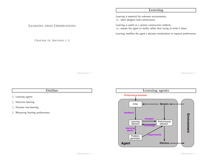
Learning agents

Performance standard

Agent Environment

Sensors Effectors Performance element changes knowledge learning goals Problem generator feedback Learning element Critic experiments

Chapter 18, Sections 1–3 4

Learning element

Design of learning element is dictated by ♦ what type of performance element is used ♦ which functional component is to be learned ♦ how that functional compoent is represented ♦ what kind of feedback is available Example scenarios:

Performance element Alpha−beta search Logical agent Simple reflex agent Component

• Eval. fn.

Transition model Transition model Representation Weighted linear function Successor−state axioms Neural net Dynamic Bayes net Utility−based agent Percept−action fn Feedback Outcome Outcome Win/loss Correct action

Supervised learning: correct answers for each instance Reinforcement learning: occasional rewards

Chapter 18, Sections 1–3 5

Inductive learning (a.k.a. Science)

Simplest form: learn a function from examples (tabula rasa) f is the target function An example is a pair x, f(x), e.g., O O X X X , +1 Problem: find a(n) hypothesis h such that h ≈ f given a training set of examples (This is a highly simplified model of real learning: – Ignores prior knowledge – Assumes a deterministic, observable “environment” – Assumes examples are given – Assumes that the agent wants to learn f—why?)

Chapter 18, Sections 1–3 6

Inductive learning method

Construct/adjust h to agree with f on training set (h is consistent if it agrees with f on all examples) E.g., curve fitting:

x f(x)

Chapter 18, Sections 1–3 7

Inductive learning method

Construct/adjust h to agree with f on training set (h is consistent if it agrees with f on all examples) E.g., curve fitting:

x f(x)

Chapter 18, Sections 1–3 8

Inductive learning method

Construct/adjust h to agree with f on training set (h is consistent if it agrees with f on all examples) E.g., curve fitting:

x f(x)

Chapter 18, Sections 1–3 9

Inductive learning method

Construct/adjust h to agree with f on training set (h is consistent if it agrees with f on all examples) E.g., curve fitting:

x f(x)

Chapter 18, Sections 1–3 10

Inductive learning method

Construct/adjust h to agree with f on training set (h is consistent if it agrees with f on all examples) E.g., curve fitting:

x f(x)

Chapter 18, Sections 1–3 11

Inductive learning method

Construct/adjust h to agree with f on training set (h is consistent if it agrees with f on all examples) E.g., curve fitting:

x f(x)

Ockham’s razor: maximize a combination of consistency and simplicity

Chapter 18, Sections 1–3 12

Attribute-based representations

Examples described by attribute values (Boolean, discrete, continuous, etc.) E.g., situations where I will/won’t wait for a table:

Example Attributes Target Alt Bar Fri Hun Pat Price Rain Res Type Est WillWait X1 T F F T Some $$$ F T French 0–10 T X2 T F F T Full $ F F Thai 30–60 F X3 F T F F Some $ F F Burger 0–10 T X4 T F T T Full $ F F Thai 10–30 T X5 T F T F Full $$$ F T French >60 F X6 F T F T Some $$ T T Italian 0–10 T X7 F T F F None $ T F Burger 0–10 F X8 F F F T Some $$ T T Thai 0–10 T X9 F T T F Full $ T F Burger >60 F X10 T T T T Full $$$ F T Italian 10–30 F X11 F F F F None $ F F Thai 0–10 F X12 T T T T Full $ F F Burger 30–60 T

Classification of examples is positive (T) or negative (F)

Chapter 18, Sections 1–3 13

Decision trees

One possible representation for hypotheses E.g., here is the “true” tree for deciding whether to wait:

No Yes No Yes No Yes No Yes No Yes No Yes None Some Full >60 30−60 10−30 0−10 No Yes

Alternate? Hungry? Reservation? Bar? Raining? Alternate? Patrons? Fri/Sat? WaitEstimate? F T F T T T F T T F T T F

Chapter 18, Sections 1–3 14

Expressiveness

Decision trees can express any boolean function of the input attributes. E.g., for Boolean attributes, truth table row → path to leaf:

F T A B F T B

A B A xor B F F F F T T T F T T T F

F F F T T T

Trivially, there is a consistent decision tree for any training set w/ one path to leaf for each example (unless f nondeterministic in x) but it probably won’t generalize to new examples Prefer to find more compact decision trees

Chapter 18, Sections 1–3 15

Hypothesis spaces

How many distinct decision trees with n Boolean attributes??

Chapter 18, Sections 1–3 16

Hypothesis spaces

How many distinct decision trees with n Boolean attributes?? = number of Boolean functions

Chapter 18, Sections 1–3 17

Hypothesis spaces

How many distinct decision trees with n Boolean attributes?? = number of Boolean functions = number of distinct truth tables with 2n rows

Chapter 18, Sections 1–3 18

Hypothesis spaces

How many distinct decision trees with n Boolean attributes?? = number of Boolean functions = number of distinct truth tables with 2n rows = 22n

Chapter 18, Sections 1–3 19

Hypothesis spaces

How many distinct decision trees with n Boolean attributes?? = number of Boolean functions = number of distinct truth tables with 2n rows = 22n E.g., with 6 Boolean attributes, there are 18,446,744,073,709,551,616 trees

Chapter 18, Sections 1–3 20

Hypothesis spaces

How many distinct decision trees with n Boolean attributes?? = number of Boolean functions = number of distinct truth tables with 2n rows = 22n E.g., with 6 Boolean attributes, there are 18,446,744,073,709,551,616 trees How many purely conjunctive hypotheses (e.g., Hungry ∧ ¬Rain)??

Chapter 18, Sections 1–3 21

Hypothesis spaces

How many distinct decision trees with n Boolean attributes?? = number of Boolean functions = number of distinct truth tables with 2n rows = 22n E.g., with 6 Boolean attributes, there are 18,446,744,073,709,551,616 trees How many purely conjunctive hypotheses (e.g., Hungry ∧ ¬Rain)?? Each attribute can be in (positive), in (negative), or out ⇒ 3n distinct conjunctive hypotheses

Chapter 18, Sections 1–3 22

Hypothesis spaces

How many distinct decision trees with n Boolean attributes?? = number of Boolean functions = number of distinct truth tables with 2n rows = 22n E.g., with 6 Boolean attributes, there are 18,446,744,073,709,551,616 trees How many purely conjunctive hypotheses (e.g., Hungry ∧ ¬Rain)?? Each attribute can be in (positive), in (negative), or out ⇒ 3n distinct conjunctive hypotheses More expressive hypothesis space – increases chance that target function can be expressed – increases number of hypotheses consistent w/ training set ⇒ may get worse predictions

Chapter 18, Sections 1–3 23

Decision tree learning

Aim: find a small tree consistent with the training examples Idea: (recursively) choose “most significant” attribute as root of (sub)tree

function DTL(examples, attributes, default) returns a decision tree if examples is empty then return default else if all examples have the same classification then return the classification else if attributes is empty then return Mode(examples) else best ← Choose-Attribute(attributes,examples) tree ← a new decision tree with root test best for each value vi of best do examplesi ← {elements of examples with best = vi} subtree ← DTL(examplesi,attributes − best,Mode(examples)) add a branch to tree with label vi and subtree subtree return tree

Chapter 18, Sections 1–3 24

Choosing an attribute

Idea: a good attribute splits the examples into subsets that are (ideally) “all positive” or “all negative”

None Some Full

Patrons?

French Italian Thai Burger

Type?

Chapter 18, Sections 1–3 25

Information Theory

♦ Consider communicating two messages (T and F) between two parties ♦ Bits are used to measure message size ♦ If P(T) = 1 and P(F) = 0, how many bits are needed? ♦ If P(T) = .5 and P(F) = .5, how many bits are needed?

Chapter 18, Sections 1–3 26

Information Theory

♦ Consider communicating two messages (T and F) between two parties ♦ Bits are used to measure message size ♦ If P(T) = 1 and P(F) = 0, how many bits are needed? ♦ If P(T) = .5 and P(F) = .5, how many bits are needed? ♦ Information: I(P(v1), ...P(vn)) =

n

i=1 −P(vi) log2 P(vi)

♦ I(1, 0) = 0 bit ♦ I(0.5, 0.5) = −0.5 × log2 0.5 − 0.5 × log2 0.5 = 1 bit

Chapter 18, Sections 1–3 27

Information Theory

♦ Consider communicating two messages (T and F) between two parties ♦ Bits are used to measure message size ♦ If P(T) = 1 and P(F) = 0, how many bits are needed? ♦ If P(T) = .5 and P(F) = .5, how many bits are needed? ♦ Information: I(P(v1), ...P(vn)) =

n

i=1 −P(vi) log2 P(vi)

♦ I(1, 0) = 0 bit ♦ I(0.5, 0.5) = −0.5 × log2 0.5 − 0.5 × log2 0.5 = 1 bit ♦ I measures the information content for communication (or uncertainty in what is already known) ♦ The more one knows, the less to be communicated, the smaller is I ♦ The less one knows, the more to be communicated, the larger is I

Chapter 18, Sections 1–3 28

Using Information Theory

♦ (P(pos), P(neg)): probabilities of positive (“message T”) and negative (“message F”) ♦ Attribute color: black (1,0), white (0,1) ♦ Attribute size: large (.5,.5), small (.5,.5)

Chapter 18, Sections 1–3 29

Before adding an attribute

♦ How much uncertainty/confusion before adding an attribute (e.g., color)?

• p = number of positive examples, n = number of negative examples
• Estimating probabilities: P(pos) =

p p+n, P(neg) = n p+n

• Before() = I(P(pos), P(neg))

Chapter 18, Sections 1–3 30

After adding an attribute

♦ How much uncertainty/confusion after adding an attribute (e.g., color)?

• pi = number of positive examples for value i (e.g., black), ni = number
• f negative ones
• Estimating probabilities for value i: Pi(pos) =

pi pi+ni, Pi(neg) = ni pi+ni

• Uncertainty from value i: I(Pi(pos), Pi(neg))
• But we have v values for attribute A (e.g., 2 for color)
• How do we combine the uncertainty from the different attribute values?

Chapter 18, Sections 1–3 31

After adding an attribute

♦ How much uncertainty/confusion after adding an attribute (e.g., color)?

• pi = number of positive examples for value i (e.g., black), ni = number
• f negative ones
• Estimating probabilities for value i: Pi(pos) =

pi pi+ni, Pi(neg) = ni pi+ni

• Uncertainty from value i: I(Pi(pos), Pi(neg))
• But we have v values for attribute A (e.g., 2 for color)
• How do we combine the uncertainty from the different attribute values?
• Remainder(A) = After(A) =

v

i=1 pi+ni p+n I(Pi(pos), Pi(neg)) [expected

uncertanity]

Chapter 18, Sections 1–3 32

Choosing an Attribute

♦ “Information Gain” (reduction in uncertainty)

• Gain(A) = Before() − After(A)
• Why Before() − After(A), not After(A) − Before() ?

Chapter 18, Sections 1–3 33

Choosing an Attribute

♦ “Information Gain” (reduction in uncertainty)

• Gain(A) = Before() − After(A)
• Why Before() − After(A), not After(A) − Before() ?
• Before() should have more uncertainty
• Choose attribute A with the largest Gain(A)

Chapter 18, Sections 1–3 34

Example contd.

Decision tree learned from the 12 examples:

No Yes

Fri/Sat?

None Some Full

Patrons?

No Yes

Hungry? Type?

French Italian Thai Burger

F T T F F T F T

Substantially simpler than “true” tree—a more complex hypothesis isn’t jus- tified by small amount of data

Chapter 18, Sections 1–3 35

Performance measurement

How do we know that h ≈ f?

Chapter 18, Sections 1–3 36

Performance measurement

How do we know that h ≈ f? How about measuring the accuracy of h on the examples that were used to learn h?

Chapter 18, Sections 1–3 37

Performance measurement

How do we know that h ≈ f? (Hume’s Problem of Induction)

• 1. Use theorems of computational/statistical learning theory
• 2. Try h on a new test set of examples
• use same distribution over example space as training set
• divide into two disjoint subsets: training and test sets
• prediction accuracy: accuracy on the (unseen) test set

Chapter 18, Sections 1–3 38

Performance measurement

Learning curve = % correct on test set as a function of training set size

0.4 0.5 0.6 0.7 0.8 0.9 1 0 10 20 30 40 50 60 70 80 90100 % correct on test set Training set size

Chapter 18, Sections 1–3 39

Learning curve

• realizable (can express target function) vs. non-realizable

non-realizability can be due to: – missing attributes – and/or restricted hypothesis class (e.g., thresholded linear function)

• redundant expressiveness (e.g., loads of irrelevant attributes)

% correct # of examples 1 nonrealizable redundant realizable

Chapter 18, Sections 1–3 40

Irrelevant Attributes

• Consider adding the attribute: Date (month and day)
• How can it affect the learned tree?

Chapter 18, Sections 1–3 41

Overfitting

• More attributes ⇒ larger hypothesis space
• Larger hypothesis space can lead to more hypotheses that represent mean-

ingless “regularity/patterns”

• Overfitting: high accuracy on training set, but low accuracy on test set—

low prediction accuracy

• Select the attribute with the largest information gain

– however, is the gain significant? – (statistical) significance test

• Pruning

– do not include the attribute if information gain is not statistically sig- nificant – potentially, less than 100% accurate on the training set, why? – however, improved prediction accuracy on the test set

Chapter 18, Sections 1–3 42

Significance Test

• “Null hypothesis” (in statistics): attribute is irrelevant (gain is not sig-

nificant)

• “Alternative hypothesis”: attribute is relevant
• Calculating the deviation

– expected ˆ pi = p × pi+ni

p+n

– expected ˆ ni = n × pi+ni

p+n

– Deviation (from expected): D =

v

• i=1

(pi − ˆ pi)2 ˆ pi + (ni − ˆ ni)2 ˆ ni – D is χ2 (chi-squared) distributed with v − 1 degrees of freedom – χ2 Test in statistics

• With a confidence level (e.g. 95%), if D > χ2 value, attribute is relevant

(Null hypothesis is rejected)

Chapter 18, Sections 1–3 43

Additional Issues

♦ Missing attribute values. ♦ Gain() biases to attributes with more values. ♦ Continuous-valued (numeric) attributes have infinite number of values.

Chapter 18, Sections 1–3 44

Learning as search

♦ What is the state space in learning decision trees? ♦ State-space formulation

Chapter 18, Sections 1–3 45

Learning as search

♦ What is the state space in learning decision trees? ♦ State-space formulation

• State: a decision tree
• Initial state: an empty decision tree
• Action: add an attribute to the tree
• Goal test: all examples in each leaf have the same classification

♦ What kind of search is DTL?

Chapter 18, Sections 1–3 46

Summary

Learning needed for unknown environments, lazy designers Learning agent = performance element + learning element Learning method depends on type of performance element, available feedback, type of component to be improved, and its representation For supervised learning, the aim is to find a simple hypothesis that is approximately consistent with training examples Decision tree learning using information gain Learning performance = prediction accuracy measured on test set

Chapter 18, Sections 1–3 47