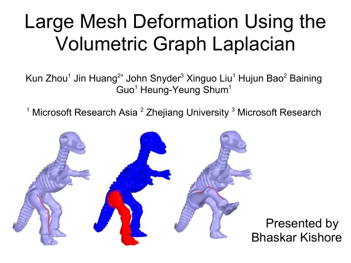
Large Mesh Deformation Using the Volumetric Graph Laplacian Kun Zhou - - PowerPoint PPT Presentation

Large Mesh Deformation Using the Volumetric Graph Laplacian

Kun Zhou1 Jin Huang2∗ John Snyder3 Xinguo Liu1 Hujun Bao2 Baining Guo1 Heung-Yeung Shum1

1 Microsoft Research Asia 2 Zhejiang University 3 Microsoft Research

Presented by Bhaskar Kishore

11/21/2007 Bhaskar Kishore 2

Outline

• Introduction
• Related Work
• Deformation on Volumetric Graphs
• Deformation from 2D curves
• Results
• Conclusions

11/21/2007 Bhaskar Kishore 3

Outline

• Introduction
• Related Work
• Deformation on Volumetric Graphs
• Deformation from 2D curves
• Results
• Conclusions

11/21/2007 Bhaskar Kishore 4

Introduction

• Large deformations

are challenging

• Existing techniques
• ften produce

implausible results

• Observation

– Unnatural volume

changes

– Local Self Intersection

11/21/2007 Bhaskar Kishore 5

Introduction

• Volumetric Graph Laplacian

– Represent volumetric details as difference between

each point in a 3D volume and the average of its neighboring points in a graph.

– Produces visually pleasing deformation results – Preserves surface details

• VGL can impose volume constraints
• Volumetric constraints are represented by a

quadric energy function

11/21/2007 Bhaskar Kishore 6

Introduction

• Volumetric Graph Laplacian

– Represent volumetric details as difference between

each point in a 3D volume and the average of its neighboring points in a graph.

– Produces visually pleasing deformation results – Preserves surface details

• VGL can impose volume constraints
• Volumetric constraints are represented by a

quadric energy function

11/21/2007 Bhaskar Kishore 7

Introduction

• To apply VGL to a triangle mesh

– Construct a volumetric graph which includes

• Points on the original mesh
• Points derived from a simple lattice lying inside the mesh

– Points are connected by graph edges which are a

superset of the edges of the original mesh

• Whats nice is that there is no need for

volumetric tessellation.

• Deformations are specified by identifying a

limited set of points – say a curve

11/21/2007 Bhaskar Kishore 8

Introduction

• This curve can then be deformed to specify

destination

• A quadric energy function is generated

– Minimum maps the points to their specified

destination

– While preserving surface detail and roughly volume

too

11/21/2007 Bhaskar Kishore 9

Introduction

• Contribution

– Demonstrate that problem of large deformation can

be effectively solved by volumetric differential

• perator
• Surface operators can be extended to solids by defining

them on tetrahedral mesh

• But that is difficult, constructing the tetrahedral mesh is

hard

• Existing packages remesh geometry and change

connectivity

– That a volumetric operator can be applied to the

easy to build Volumetric graph without meshing int.

11/21/2007 Bhaskar Kishore 10

Outline

• Introduction
• Related Work
• Deformation on Volumetric Graphs
• Deformation from 2D curves
• Results
• Conclusions

11/21/2007 Bhaskar Kishore 11

Related Work

• Freeform modeling [Botsch Kobbelt 2004]
• Curve based FFD [ Sing and Fiume 1998]
• Lattice based FFD [ Sederberg and Parry 1986]
• Displacement volumes [Botsch and Kobbelt

2003]

• Poisson meshes [Yu et al 2004]

11/21/2007 Bhaskar Kishore 12

Outline

• Introduction
• Related Work
• Deformation on Volumetric Graphs
• Deformation from 2D curves
• Results
• Conclusions

11/21/2007 Bhaskar Kishore 13

Deformation on Volumetric Graphs

• Let M = (V, K) be a triangular mesh

– V = {pi ϵ R3 | 1≤ i ≤ n}, is a set of n point position – K is a abstract simplicial complex containing three

types of elements

• Vertices {i}
• Edges {i,j}
• Faces {i,j,k}

11/21/2007 Bhaskar Kishore 14

Laplacian Deformation on Abstract Graphs

• Suppose G = (P,E) is a graph

– P {pi ϵ R3 | 1≤ i ≤ N}, is a set of N point positions – E = {(i,j) | pi is connected to pj}

• Then Laplacian coordinate δi of a point pi

where N (i) = { j |{i, j} ∈ E}

• LG is called the Laplace operator on graph G

11/21/2007 Bhaskar Kishore 15

Laplacian Deformation on Abstract Graphs

• To control the deformation

– User inputs deformed positions qi, i ∈ { 1, ..., m} for

a subset of the N mesh vertices

– Compute a new (deformed) laplacian coordinate δ'i

for each point i in the graph

– Deformed positions of the mesh vertices p'i is

• btained by solving

11/21/2007 Bhaskar Kishore 16

Laplacian Deformation on Abstract Graphs

• The first term represents preservation of local

detail

• The second term constrains the position of

those vertices directly specified by the user

• Alpha is used to balance these two objectives

11/21/2007 Bhaskar Kishore 17

Laplacian Deformation on Abstract Graphs

• Deformed Laplacian coordinates are computed

via δ ′i = Ti δi

• δi is the Laplacian in rest pose
• δ ′i is the Laplacian in the deformed pose
• Ti is restricted to rotation and isotropic scale
• Local transforms are propagated from the

deformed region to the entire mesh

11/21/2007 Bhaskar Kishore 18

Constructing a Volumetric Graph

• Build two graphs, Gin and Gout
• Gin prevents large volume changes
• Gout prevents local self-intersection
• Gin can obtained by tetrahedralizing the interior

– Difficult to implement – Computationally expensive – Produces poorly shaped tetrahedra for complex

models

11/21/2007 Bhaskar Kishore 19

Constructing a Volumetric Graph

• Build two graphs, Gin and Gout
• Gin prevents large volume changes
• Gout prevents local self-intersection
• Gin can obtained by tetrahedralizing the interior

– Difficult to implement – Computationally expensive – Produces poorly shaped tetrahedra for complex

models

11/21/2007 Bhaskar Kishore 20

Constructing the Volumetric Graph

• Algorithm

– Construct inner shell Min for mesh M by offsetting

each vertex a distance in the direction opposite to its Normal

– Embed Min and M in a body-centered cubic lattice.

Remove lattice nodes outside of Min

– Build edge connections among M, Min, and lattice

nodes

– Simplify the graph using edge collapse and smooth

the graph

11/21/2007 Bhaskar Kishore 21

Constructing the Volumetric Graph

• Construct inner shell Min for mesh M by
• ffsetting each vertex a distance in the direction
• pposite to its Normal

11/21/2007 Bhaskar Kishore 22

Constructing the Volumetric Graph

• Embed Min and M in a body-centered cubic
• lattice. Remove lattice nodes outside of Min

11/21/2007 Bhaskar Kishore 23

Constructing the Volumetric Graph

• Build edge connections among M, Min, and

lattice nodes

11/21/2007 Bhaskar Kishore 24

Constructing the Volumetric Graph

• Simplify the graph using edge collapse and

smooth the graph

11/21/2007 Bhaskar Kishore 25

Constructing the Volumetric Graph

• Min ensures that inner points are inserted even

in thin features that may be missed by lattice sampling.

• Question : how much of a step should one take

to construct Min?

• Use iterative method based on simplification

envelopes [Cohen et al. 1996]

11/21/2007 Bhaskar Kishore 26

Constructing the Volumetric Graph

• Min ensures that inner points are inserted even

in thin features that may be missed by lattice sampling.

• Question : how much of a step should one take

to construct Min?

– Use iterative method based on simplification

envelopes [Cohen et al. 1996]

11/21/2007 Bhaskar Kishore 27

Constructing the Volumetric Graph

• Use iterative method based on simplification

envelopes [Cohen et al. 1996]

– At each iteration

• Move each vertex a fraction of the average edge length
• Test its adjacent triangles for intersection with each other

and the rest of the model

• If no intersections are found, accept step, else reject it
• Iterations terminate when all vertices have moved desired

distance or can no longer move

11/21/2007 Bhaskar Kishore 28

Constructing the Volumetric Graph

• Use iterative method based on simplification

envelopes [Cohen et al. 1996]

– At each iteration

• Move each vertex a fraction of the average edge length
• Test its adjacent triangles for intersection with each other

and the rest of the model

• If no intersections are found, accept step, else reject it
• Iterations terminate when all vertices have moved desired

distance or can no longer move

11/21/2007 Bhaskar Kishore 29

Constructing the Volumetric Graph

• The BCC lattice

– Consists of nodes at every point of a Cartesian grid – Additionally there are nodes at cell centers – Node locations may be viewed as belong to two

interlaced grids

– This lattice provides desirable rigidity properties as

seen in crystalline structures in nature

– Grid interval set to average edge length

11/21/2007 Bhaskar Kishore 30

Constructing the Volumetric Graph

• Three types of edge connections for an initial

graph

– Each vertex in M is connected to its corresponding

vertex in Min. Shorter diagonal for each prism face is included as well.

– Each inner node of the BCC lattice is connected with its

eight nearest neighbors in the other interlaced grid

– Connections are made between Min and nodes of the

BCC lattice.

• For each edge in the BCC lattice that intersects Min and

has at least one node inside Min, we connect the BCC lattice node inside Min to the point in Min closest to this intersection

11/21/2007 Bhaskar Kishore 31

Constructing the Volumetric Graph

• Three types of edge connections for an initial

graph

– Each vertex in M is connected to its corresponding

vertex in Min. Shorter diagonal for each prism face is included as well.

– Each inner node of the BCC lattice is connected with its

eight nearest neighbors in the other interlaced grid

– Connections are made between Min and nodes of the

BCC lattice.

• For each edge in the BCC lattice that intersects Min and

has at least one node inside Min, we connect the BCC lattice node inside Min to the point in Min closest to this intersection

11/21/2007 Bhaskar Kishore 32

Constructing the Volumetric Graph

• Simplification and Smoothing

– Visit graph in increasing order of length – If length of an edge is less than a threshold,

collapse it to edge's mid point

• Threshold is half of average edge length of M

– Apply iterative smoothing

• Each point is moved to the average of its neighbors
• Three smoothing operations in their implementation

– No smoothing or simplification are applied to the

vertices of original mesh M

11/21/2007 Bhaskar Kishore 33

Constructing the Volumetric Graph

• Gout can be constructed in a similar way to Gin
• Mout can be obtained by moving a small step in

the normal direction.

• Connections for Mout can be made similar Min
• Intersections between Min and Mout and with M

can occur, especially in meshes containing regions of high curvature.

– They claim it does not cause any difficulty in our

interactive system.

11/21/2007 Bhaskar Kishore 34

Deforming the Volumetric Graph

• We modify equation (2) to include volumetric

constraints

Where the first n points in graph G belong the mesh M

– G' is a sub-graph of G formed by removing those edges belonging

to M

– δ ′i (1 ≤ i ≤ N) in G' are the graph laplcians coordinates in the

deformed frame.

– For points in the original mesh M, ε' (1 ≤ i ≤ n) are the mesh

laplacian coordinates in the deformed coordinate frame

11/21/2007 Bhaskar Kishore 35

Deforming the Volumetric Graph

• – β balances between surface and volumetric detail

where β = nβ'/N.

– The n/N factor normalizes the weight so that it is

insensitive to the lattice density

– β' = 1 works well – α is not normalized – We want constraint strength to

depend on the number of constrained points relative to the total number of mesh points

• 0.1 < α < 1, default is 0.2

11/21/2007 Bhaskar Kishore 36

Propagation of Local Transforms

• Local Transforms take the Laplacian

coordinates in the rest frame to the deformed frame

• Use WIRE deformation method [Singh and

Flume]

• Select a sequence of mesh vertices forming a

curve

• Deform the curve.

11/21/2007 Bhaskar Kishore 37

Propagation of Local Transforms

• First determine where neighboring graph points

deform to, then infers local transforms at the curve points, finally propagate the transforms

• ver the whole mesh
• Begin by finding mesh neighbors of qi and
• btain their deformed positions using WIRE.
• Let C(u) and C'(u) be the original curve and the

deformed curves parametrized by arc length u = [0,1]

11/21/2007 Bhaskar Kishore 38

Propagation of Local Transforms

• Given some neighboring point p ϵ R3, let up ϵ

[0,1] be the parameter vale minimizing distnace between p and the curve c(u).

• The deformation mapping p to p' such that C

maps to C' is given by

• R is a 3x3 rotation matrix taking the tangent

vector t(u) on C and maps it to t'(u) on C' by rotating around t(u)xt'(u)

11/21/2007 Bhaskar Kishore 39

Propagation of Local Transforms

• s(u) is a scale factor

– Computed at each curve vertex as the ratio of the

sum of lengths of its adjacent edges in C' over this length in C

– It is then defined continuously over u by liner

interpolation

• Above equation gives us deformed coordinates

for each point in the curve and its 1 Ring neighborhood

11/21/2007 Bhaskar Kishore 40

Propagation of Local Transforms

• Transformations are propagated from the

control curve to all graph points p via a deformation strength field f(p)

• f(p) decays away from the deformation site.

– Constant – Linear – Gaussian – Based on shortest edge path from p to the curve

11/21/2007 Bhaskar Kishore 41

Propagation of Local Transforms

• A rotation is defined by

– Computing a normal and tangent vector as the

perpendicular projection of one edge vector with this normal

– Normal is computed as a linear combination

weighted by face area of face normals around mesh point i

– Rotation is represented as a quaternion

• Angle should be less than 180

11/21/2007 Bhaskar Kishore 42

Propagation of Local Transforms

• The simplest propagation scheme is to assign

to p a rotation and scale from the point qp on the control curve closest to p

• Smoother results are obtained by computing a

weighted average over all the vertices on the control curve instead of the closest

11/21/2007 Bhaskar Kishore 43

Propagation of Local Transforms

• Weighting over multiple curves is similar, we

accumulate values over multiple curves

• Final transformation matrix is given by

11/21/2007 Bhaskar Kishore 44

Propagation of Local Transforms

11/21/2007 Bhaskar Kishore 45

Weighting Scheme

• They drop uniform weighting in favor of another

scheme that provides better results

• For mesh Laplacian Lm, use cotangent weights
• For graph Laplacian, compute weights by

solving a quadratic programming problem

11/21/2007 Bhaskar Kishore 46

Weighting Scheme

• For each graph vertex i, to obtain weights wij

solve

– The first term generates Laplacian coordinates of smallest magnitude – Second term is based on scale dependent umbrella operator which

prefers weight in proportion to inverse of edge length

– Lamba balances the two objects (set to 0.01) – Zeta prevents small weights (set to 0.01)

11/21/2007 Bhaskar Kishore 47

Weighting Scheme

11/21/2007 Bhaskar Kishore 48

Quadric Energy Minimization

• To minimize energy in equation (3) we solve the

following equations

– Above equations represent a sparse linear system Ax = b – Matrix A is only dependent on the original graph and A- can be

precomputed using LU decomposition

– B depends on current Laplacian coordinates and changes during

interactive deformation

11/21/2007 Bhaskar Kishore 49

Multi resolution Methods

• Solving a the linear system of a large complex

model is expensive

• Generate a simplified mesh [Guskov et al.

1999]

• Deform this mesh and then add back the details

to obtain high resolution deformed mesh

11/21/2007 Bhaskar Kishore 50

Outline

• Introduction
• Related Work
• Deformation on Volumetric Graphs
• Deformation from 2D curves
• Results
• Conclusions

11/21/2007 Bhaskar Kishore 51

Deformation from 2D curves

• Method

– User defines control curve by selecting sequence

points on the mesh which are connected by the shortest edge path (dijkstra)

– This 3D curve is projected onto one or more planes – Editing is done in these planes – The deformed curve is projected back into 3D,

which then forms the basis of the deformation process

11/21/2007 Bhaskar Kishore 52

Deformation from 2D curves

• Curve Projection

– Given a curve, the system automatically selects projection

planes base on its average normal and principal vectors.

– Principal vectors are computed as the two eigen vectors

corresponding to the largest eigen values from a principal component analysis

– In most cases, cross product of the average normal and the

first principal vector provide a satisfactory plane

– If length of average normal vector is small, then use only two

principal vectors instead

11/21/2007 Bhaskar Kishore 53

Deformation from 2D curves

• Curve Editing

– Projected 2D curves inherit geometric detail from original

mesh that complicates editing

– They use an editing method for discrete curves base on

Laplacian coordinates

– Laplacian coordinate of a curve vertex is the difference

between its position and the average position of its neighbors or a single neighbor in cases of terminal vertices

– Denote the 2D curve to be edited as C – A cubic B-Spline curve Cb is first computed as a least

squares fit to C. This represents the low frequencies of C

11/21/2007 Bhaskar Kishore 54

Deformation from 2D curves

• Curve Editing

– A discrete version of Cb , Cd is computed by mapping each

vertex of C onto Cb using proportional arc length mapping

– We can not edit the discrete version conveniently – After editing we obtain C'b and C'd . These curves lack the

• riginal detail of the Cb

– To restore detail, at each vertex of C we find a the unique

rotation and scale that maps its location from Cd to C'd

– Applying these transformations to the Laplacian coordinates

and solving equation (2) without the constraint term

11/21/2007 Bhaskar Kishore 55

Deformation from 2D curves

• Deformation Re-targeting from 2D Cartoons

– An application of 2D sketch based deformation – Users specify one or more 3D control curves on the mesh along

with their project planes and for each curves a series of 2D curves in the cartoon image sequence that drive its deformation

– It is not necessary to generate a deformation from scratch at

every time frame. Users can select a curves in a few key frames

• f the cartoon

– Automatic interpolation technique based on differential

coordinates is used to interpolate between key frame

11/21/2007 Bhaskar Kishore 56

Deformation from 2D curves

• Deformation Re-targeting from 2D Cartoons

– Say we have two meshes M and M' at two different key frames – Compute the Laplacian coordinates for each vertex in the two

meshes

– A rotation and scale in the local neighborhood of each vertex p is

computed taking the Laplacian coordinates from its location in M to M'

– Denote the transform as Tp. Interpolate Tp over time to transition

from M to M'

– 2D cartoon curves are deformed in a single plane, this allows for

extra degrees of freedom if required by the user

11/21/2007 Bhaskar Kishore 57

Deformation from 2D curves

• Deformation Re-targeting from 2D Cartoons

11/21/2007 Bhaskar Kishore 58

Deformation from 2D curves

• Deformation Re-targeting from 2D Cartoons

11/21/2007 Bhaskar Kishore 59

Outline

• Introduction
• Related Work
• Deformation on Volumetric Graphs
• Deformation from 2D curves
• Results
• Conclusions

11/21/2007 Bhaskar Kishore 60

Results

• Some stats

11/21/2007 Bhaskar Kishore 61

More results

11/21/2007 Bhaskar Kishore 62

More results

11/21/2007 Bhaskar Kishore 63

Outline

• Introduction
• Related Work
• Deformation on Volumetric Graphs
• Deformation from 2D curves
• Results
• Conclusions

11/21/2007 Bhaskar Kishore 64

Conclusions

• They proposed a system which would address

volumetric changes and local self intersection based on the volumetric graph Laplacian

• The solution avoids the intricacies of solidly

meshing complex objects

• Presented a system for retargetting 2D

animations to 3D

• Note, that their system does not address global

self intersections – those must addressed by the user