Lab 2: 12 th March 2012 Exercise 1: Probabilistic Models Lets - PDF document

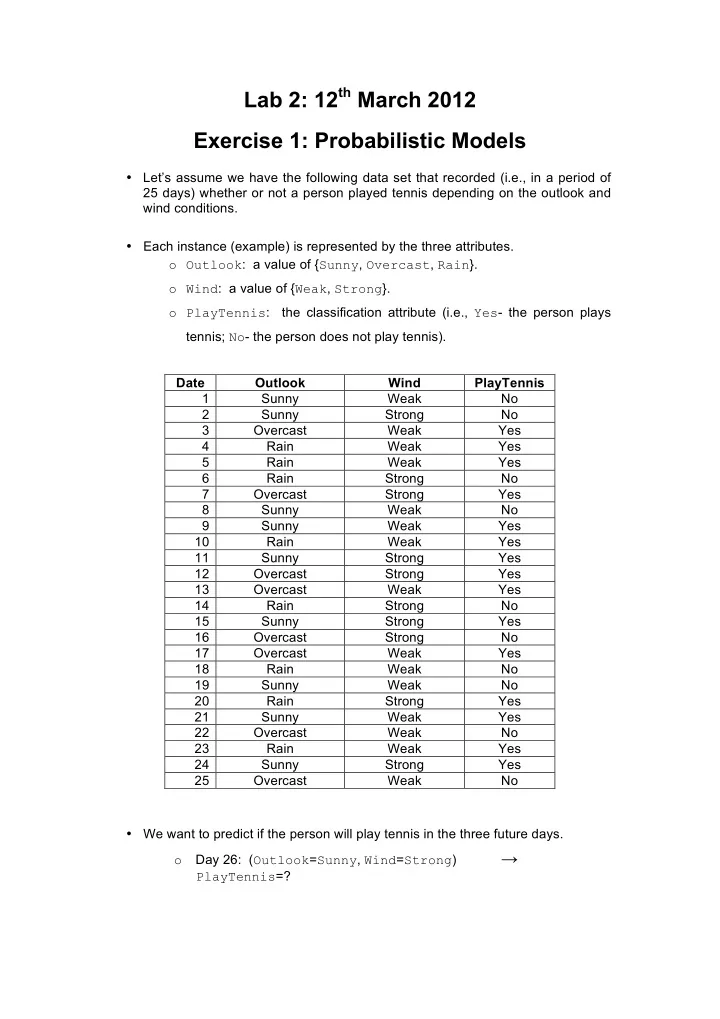
Lab 2: 12 th March 2012 Exercise 1: Probabilistic Models • Let’s assume we have the following data set that recorded (i.e., in a period of 25 days) whether or not a person played tennis depending on the outlook and wind conditions. • Each instance (example) is represented by the three attributes. o Outlook : a value of { Sunny , Overcast , Rain }. o Wind : a value of { Weak , Strong }. o PlayTennis : the classification attribute (i.e., Yes - the person plays tennis; No - the person does not play tennis). Date Outlook Wind PlayTennis 1 Sunny Weak No 2 Sunny Strong No 3 Overcast Weak Yes 4 Rain Weak Yes 5 Rain Weak Yes 6 Rain Strong No 7 Overcast Strong Yes 8 Sunny Weak No 9 Sunny Weak Yes 10 Rain Weak Yes 11 Sunny Strong Yes 12 Overcast Strong Yes 13 Overcast Weak Yes 14 Rain Strong No 15 Sunny Strong Yes 16 Overcast Strong No 17 Overcast Weak Yes 18 Rain Weak No 19 Sunny Weak No 20 Rain Strong Yes 21 Sunny Weak Yes 22 Overcast Weak No 23 Rain Weak Yes 24 Sunny Strong Yes 25 Overcast Weak No • We want to predict if the person will play tennis in the three future days. → o Day 26: ( Outlook = Sunny , Wind = Strong ) PlayTennis =?

→ o Day 27: ( Outlook = Overcast , Wind = Weak ) PlayTennis =? → o Day 28: ( Outlook = Rain , Wind = Weak ) PlayTennis =? Manually compute the predictions (i.e., the person will play tennis or not) for the three future days (i.e., Days 26-28) using: • The MAP (maximum a posteriori) approach • The MLE (maximum likelihood estimation) approach • The Naïve Bayes classification approach. Solution ¡for ¡Day ¡26 ¡ ¡ MAP ¡ ! ! ℎ ! ℎ ℎ !"# = argmax ! ∈ !" , !"# ! ℎ ! = ¡ argmax ! ∈ !" , !"# ! ! = ¡ argmax ! ∈ !" , !"# ! ! ℎ ! ℎ ¡ ¡ !" ! ! ! !" = !" = ! ¡ ¡ ¡ ¡ ¡ ¡ ¡ ¡ ¡ ¡ ¡ ¡ ¡ ¡ ¡ ¡ ¡ ¡ ¡ ¡ ¡ ¡ ¡ ! !"# = ! ¡ ¡ ! !"#$!!% = !"##$ , !"#$ = !"#$%& !" = 3 15 = 1 5 ¡ ¡ ! !"#$!!% = !"##$ , !"#$ = !"#$%& !"# = 1 10 ¡ ¡ ! !"#$!!% = !"##$ , !"#$ = !"#$%& !" ∗ ! !" = 1 5 ∗ 3 5 = 3 25 = 6 50 ¡ ¡ ! !"#$!!% = !"##$ , !"#$ = !"#$%& !"# ∗ ! !"# = 1 10 ∗ 2 5 = 2 50 ¡ ¡ ! !"#$!!% = !"##$ , !"#$ = !"#$%& !" ∗ ! !" > ! !"#$!!% = !"##$ , !"#$ = !"#$%& !"# ∗ ! !"# ¡ ¡ Hence: ¡D 26 ¡ à ¡Play ¡Tennis ¡ ¡ ¡ ¡ ¡ ¡ ¡

MLE ¡ ℎ !"# = argmax ! ∈ !" , !"# ! ! ℎ ¡ ¡ ! !"#$!!% = !"##$ , !"#$ = !"#$%& !" = 1 5 = 2 10 ¡ ¡ ! !"#$!!% = !"##$ , !"#$ = !"#$%& !"# = 1 10 ¡ ¡ ! !"#$!!% = !"##$ , !"#$ = !"#$%& !" > ! !"#$!!% = !"##$ , !"#$ = !"#$%& !"# ¡ ¡ Hence: ¡D 26 ¡ à ¡Play ¡Tennis ¡ ¡ ¡ ¡ Naïve Bayes classification ¡ ! ℎ !" = argmax ! ∈ !" , !"# ! ℎ ∗ ! ! ! ℎ = ! ! ! = argmax ! ∈ !" , !"# ! ℎ ∗ ! !"#$!!% = !"##$ ℎ ∗ ! ( !"#$ = !"#$%& | ℎ ) ¡ ¡ ¡ !" ! ! ! !" = !" = ! ¡ ¡ ¡ ¡ ¡ ¡ ¡ ¡ ¡ ¡ ¡ ¡ ¡ ¡ ¡ ¡ ¡ ¡ ¡ ¡ ¡ ¡ ¡ ¡ ¡ ¡ ¡ ¡ ¡ ¡ ¡ ¡ ¡ ¡ ¡ ¡ ¡ ¡ ¡ ¡ ¡ ¡ ¡ ¡ ¡ ! !"# = ! ¡ ¡ ! ! ! !"#$!!% = !"##$ !" = !" ¡ ¡ ¡ ¡ ¡ ¡ ¡ ¡ ¡ ¡ ¡ ¡ ¡ ¡ ¡ ¡ ¡ ! !"#$ = !"#$%& !" = !" ¡ ¡ ! ! ! !"#$!!% = !"##$ !"# = !" ¡ ¡ ¡ ¡ ¡ ¡ ¡ ¡ ¡ ¡ ¡ ¡ ¡ ! !"#$ = !"#$%& !"# = !" ¡ ¡ ! !" ∗ ! !"#$!!% = !"##$ !" ∗ ! !"#$ = !"#$%& !" = 3 5 ∗ 4 15 ∗ 6 15 = 0 . 064 ¡ ¡ ! !" ∗ ! !"#$!!% = !"##$ !"# ∗ ! !"#$ = !" !"#$ !"# = 2 5 ∗ 4 10 ∗ 4 10 = 0 . 064 ¡ ¡ The ¡ 2 ¡ hypothesis ¡ are ¡ equivalent ¡ à ¡ the ¡ decision ¡ on ¡ classification ¡ is ¡ left ¡ to ¡ a ¡ human ¡expert. ¡ ¡ ¡

¡ ¡ ¡ ¡ Exercise 2: Nearest Neighbor Learner • Assume a training set made of plant records • Each plant record (i.e., example) is represented by the 5 attributes. - SepalLength – the plant’s sepal length in cm. - SepalWidth – the plant’s sepal width in cm. - PetalLength – the plant’s petal length in cm. - PetalWidth – the plant’s petal width in cm. - Class – the classification attribute, with the possible values { Iris-setosa , Iris-versicolor, Iris-virginica }. PlantID SepalLength SepalWidth PetalLength PetalWidth Class 1 5.1 3.5 1.4 0.2 Iris-setosa 2 7.1 3.0 5.9 2.1 Iris-virginica 3 5.4 3.4 1.5 0.4 Iris-setosa 4 6.4 3.2 4.5 1.5 Iris-versicolor 5 6.3 3.3 4.7 1.6 Iris-versicolor 6 7.3 2.9 6.3 1.8 Iris-virginica 7 4.4 2.9 1.4 0.2 Iris-setosa 8 4.9 3.1 1.5 0.1 Iris-setosa 9 5.8 2.8 5.1 2.4 Iris-virginica 10 5.6 2.9 3.6 1.3 Iris-versicolor 11 6.9 3.2 5.7 2.3 Iris-virginica 12 6.0 3.4 4.5 1.6 Iris-versicolor 13 7.2 3.0 5.8 1.6 Iris-virginica 14 4.8 3.4 1.9 0.2 Iris-setosa 15 6.8 2.8 4.8 1.4 Iris-versicolor • We want to predict the class for each of the following plants. - Plant #16. ( SepalLength =4.6; SepalWidth =3.6; PetalLength =1.0; PetalWidth =0.2). - Plant #17. ( SepalLength =6.1; SepalWidth =2.8; PetalLength =4.0; PetalWidth =1.3). - Plant #18. ( SepalLength =7.7; SepalWidth =3.0; PetalLength =6.1; PetalWidth =2.3). • Manually Apply the Nearest Neighbor learning algorithm to classify the three to- be-predicted plants (i.e., Plants #16-18) – what kind of plant it is. - Try the three different values for the neighborhood size; i.e., k=1; 3; and 5.

- Use one of the geometry distance functions (e.g., Manhattan or Euclidean distance function). Solution ¡for ¡Plant ¡#16 ¡ Please see ml_2012_lab_02_nn_solution.xlsx where • md=Manhattan distance • ed = Euclidean distance • all attributes have the same weight • no normalization of distances has been done