L EAKY -wave antennas (LWAs) are electrically-long open [15], an - - PDF document

▶

Mar 04, 2023 214 likes •389 views

IEEE TRANSACTIONS ON SIGNAL PROCESSING 1 On the Use of the Z Transform of LTI Systems for the Synthesis of Steered Beams and Nulls in the Radiation Pattern of Leaky-Wave Antenna Arrays Rafael Verd u-Monedero, Jos e-Luis G omez-Tornero,

SLIDE 1

IEEE TRANSACTIONS ON SIGNAL PROCESSING 1

On the Use of the Z Transform of LTI Systems for the Synthesis of Steered Beams and Nulls in the Radiation Pattern of Leaky-Wave Antenna Arrays

Rafael Verd´ u-Monedero, Jos´ e-Luis G´

mez-Tornero, Senior Member, IEEE,

Abstract—This paper addresses the use of the Z transform to synthesize radiation patterns with prescribed nulls from a phased-array of electronically reconfigurable leaky-wave antennas (LWAs). This approach provides the relationship between such antennas and linear and time invariant (LTI) systems. Using this signal processing perspective, the proper locations of the poles and zeros of the Z transform of the associated LTI system, provide a radiation pattern with prescribed specifications (mainly main lobes directions and surrounding radiation nulls). Then, these poles and zeros positions can be transformed into particular values of the LWA array control coefficients. The effectiveness

f the proposed technique is demonstrated with the synthesis
f various radiation patterns, with application to reconfigurable

smart antennas. A comparison with more conventional uniform linear array (ULA) architecture is also performed to evaluate the synthesis flexibility and system complexity of the proposed approach. Index Terms—LTI systems, Z transform, Fourier transform, leaky-wave antennas, antenna arrays synthesis.

I. INTRODUCTION

L

EAKY -wave antennas (LWAs) are electrically-long open waveguides supporting the propagation of a travelling- wave leaky mode (LM). The LM produces continuous leakage as it propagates, creating a controlled smooth illumination

f the long radiating aperture, and then a directive scanned
radiation. The properties of leaky waves were originally

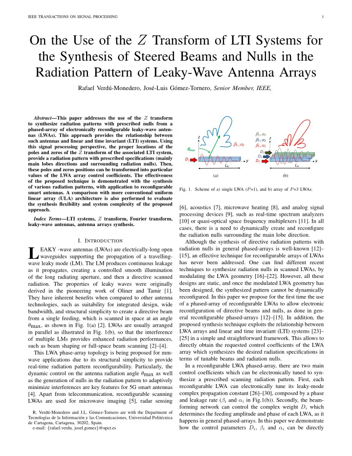
derived in the pioneering work of Oliner and Tamir [1]. They have inherent benefits when compared to other antenna technologies, such as suitability for integrated design, wide bandwidth, and structural simplicity to create a directive beam from a single feeding, which is scanned in space at an angle θmax, as shown in Fig. 1(a) [2]. LWAs are usually arranged in parallel as illustrated in Fig. 1(b), so that the interference

f multiple LMs provides enhanced radiation performances,

such as beam shaping or full-space beam scanning [2]–[4]. This LWA phase-array topology is being proposed for mm- wave applications due to its structural simplicity to provide real-time radiation pattern reconfigurability. Particularly, the dynamic control on the antenna radiation angle θmax as well as the generation of nulls in the radiation pattern to adaptively minimize interferences are key features for 5G smart antennas [4]. Apart from telecommunication, reconfigurable scanning LWAs are used for microwave imaging [5], radar sensing

R. Verd´

u-Monedero and J.L. G´

mez-Tornero are with the Department of

Tecnolog´ ıas de la Informaci´

n y las Comunicaciones, Universidad Polit´

ecnica de Cartagena, Cartagena, 30202, Spain. e-mail: {rafael.verdu, josel.gomez}@upct.es y z LA θmax D1 β1 ,α1 β α β α β α (a) D2 z θ β α y z LA D1 β3 ,α3 β2 ,α2 β1 ,α1 D3 (b)

Fig. 1. Scheme of a) single LWA (P=1), and b) array of P=3 LWAs.

[6], acoustics [7], microwave heating [8], and analog signal processing devices [9], such as real-time spectrum analyzers [10] or quasi-optical space frequency multiplexers [11]. In all cases, there is a need to dynamically create and reconfigure the radiation nulls surrounding the main lobe direction. Although the synthesis of directive radiation patterns with radiation nulls in general phased-arrays is well-known [12]– [15], an effective technique for reconfigurable arrays of LWAs has never been addressed. One can find different recent techniques to synthesize radiation nulls in scanned LWAs, by modulating the LWA geometry [16]–[22]. However, all these designs are static, and once the modulated LWA geometry has been designed, the synthesized pattern cannot be dynamically

reconfigured. In this paper we propose for the first time the use
f a phased-array of reconfigurable LWAs to allow electronic

reconfiguration of directive beams and nulls, as done in general reconfigurable phased-arrays [12]–[15]. In addition, the proposed synthesis technique exploits the relationship between LWA arrays and linear and time invariant (LTI) systems [23]– [25] in a simple and straightforward framework. This allows to directly obtain the requested control coefficients of the LWA array which synthesizes the desired radiation specifications in terms of tunable beams and radiation nulls. In a reconfigurable LWA phased-array, there are two main control coefficients which can be electronically tuned to synthesize a prescribed scanning radiation pattern. First, each reconfigurable LWA can electronically tune its leaky-mode complex propagation constant [26]–[30], composed by a phase and leakage rate (βi and αi in Fig.1(b)). Secondly, the beam- forming network can control the complex weight Di which determines the feeding amplitude and phase of each LWA, as it happens in general phased-arrays. In this paper we demonstrate how the control parameters Di, βi and αi can be directly

SLIDE 2

IEEE TRANSACTIONS ON SIGNAL PROCESSING 2

btained from the radiation pattern specifications using the

proposed synthesis technique, thanks to the special nature of LMs and their inherent relation with the impulse response of the poles of a discrete LTI system. Also, it must be noticed that LWA arrays are a particular type of phased-arrays. As it will be clarified in this paper, LWAs require less control signals and associated hardware than general uniform linear arrays (ULAs), as sketched in Fig.2. This benefit is more remarkable for long aperture arrays, as the ones requested for directive beaming and nulling. On the

ther hand, the aperture distribution of LWA arrays is more

restricted than general ULAs, which can ideally create any arbitrary radiation pattern including those generated by abrupt illumination functions. Therefore, this paper also addresses the synthesis flexibility of LWAs array in terms of other important radiation pattern features such as control of the sidelobe level (SLL), width and depth of the null region, and simultaneous synthesis of several directive scanned beams and nulls. The paper is distributed as follows. Section II is devoted to compare the proposed LWA synthesis method with related array and LWA pattern synthesis techniques. Section III starts from the well-known relationship between the radiation inte- gral and the Fourier transform. Next, we develop an original approach which links the poles and zeros of the Z transform

f a LTI system to a fixed number of LMs coexisting in a

LWA array. Section IV shows results, illustrating the pattern synthesis flexibility in terms of different radiation features, such as control on the main beam width and scanning direction, SLL reduction, tuning of the radiation nulls location, width and depth, or generation of multiple tunable beams with intermediate null regions. Finally, Section V closes the paper with the conclusions and ongoing research.

II. COMPARISON WITH RELATED SYNTHESIS TECHNIQUES

This section is dedicated to differentiate the technique proposed in this paper for LWA array synthesis with other methods which can be found in the literature. For that, we firstly compare the proposed LWA array technique with general phased arrays. Fig.2(a) shows the scheme of a general uniform linear phased-array (ULA) [12]–[15]. As explained in [31] and [32], the distance between two consecutive antennas

f the ULA must be lower than λ0/2 to satisfy the Nyquist

sampling criterion in the space domain. Otherwise, unwanted grating lobes appear due to aliasing. Therefore, a ULA with an aperture length LA needs a minimum of PULA = 2LA/λ0 + 1

antennas. As sketched in Fig.2(a), an electronically control-

lable beam-forming network must be used to distribute the RF input signal to each individual antenna element with the appropriate variable gain and phase shift. For that, each specific antenna must be fed with a variable amplifier/attenuator and a variable phase shifter to fully control the complex weighting coefficients Di. Thus, two control signals per antenna are used to adjust the amplitude and the phase of Di, namely Ai and φi in Fig.2(a). Therefore, a total of 4LA/λ0+2 control signals are needed to electronically adjust a synthesized radiation pattern in an ULA phased-array of length LA. On the other hand, the proposed LWA phased-array technique needs four control

Fig. 2. Comparison of the schemes of (a) a general uniform linear phased-

array (ULA) for array synthesis; and (b) the proposed phased-array of P reconfigurable LWAs.

signals per each LWA forming the array. As shown in Fig.2(b), two control signals are used to vary the leaky-mode phase and attenuation constants, βi and αi as explained in [26]–[29], while two control signals Ai and φi are requested to adjust the amplitude and the phase of each LWA complex weighting coefficients Di (as in conventional phased-arrays). Therefore, a total of 4P control signals are needed to implement the proposed LWA array synthesis technique for a phased-array

f P LWAs. It is important to highlight that this number of

control signals (4P) is independent on the array length LA. Therefore, for directive arrays with a long radiating aperture LA of several wavelengths as the ones treated here, a LWA array requires less amount of control signals than a general ULA of the same aperture length. For instance, for a radiating aperture length LA = 10λ0, a conventional ULA would require a total of 42 control signals. On the other hand, a LWA phased-array with the same aperture length LA = 10λ0 formed by P = 3 LWAs would require 12 control signals. Concerning the design flexibility, an array of P LWAs can create up to P individual scanned main beams, and up to P − 1 scanned radiation nulls. Also, other radiation pattern specifications such as main beam width and sidelobe level, can be adjusted with the proposed LWA array technique as it will be demonstrated thorough this paper. Still, ULAs offer the highest design flexibility since this type of antenna arrays are not restricted to any type of aperture distributions. For instance, a general ULA can synthesize an aperture distribution with abrupt changes in the amplitude and phases of the radiated fields from one antenna to the next antenna forming the array aperture. On the contrary, LWAs can only produce the type of continuous amplitude and phase aperture illuminations associated to a leaky-mode, that is, a continuous and smooth exponential decaying amplitude distribution, with linear-phase

distribution. Therefore, more abrupt aperture distributions

which can lead to other types of reconfigurable radiation patterns cannot be generally synthesized with a LWA array.

SLIDE 3

IEEE TRANSACTIONS ON SIGNAL PROCESSING 3

TABLE I COMPARISON OF SYNTHESIS TECHNIQUES FOR ARRAY PATTERNS. Refs. Antenna type Pros Cons [12]–[15], [31], [32] General uniform linear phased- array (ULA). Most flexible array synthesis. High amount of control signals for large arrays. Numerical pattern synthesis and optimization. [26]–[30] Single reconfigurable LWA. Single LWA antenna, only two control signals. Only

main beam direction and its beamwidth can be tuned. Cannot tune a radiation null. [16]–[22] Single modulated LWA (static) to generate radiation nulls. Single LWA without control signal. Can synthesize deep and wide radiation nulls. The synthesized radiation pattern (including radiation nulls) cannot be electronically tuned. [33]–[36] Single modulated LWA Single LWA without control signal. The direction of each beam cannot be electroni- (static) to generate multiple beams. Can synthesize multiple beams using a single aperture. cally scanned. This work Phased-array of P reconfigurable LWAs. Lower amount of control signals than a general linear phased-array. P LWAs are needed to tune P scanned beams and P − 1 steered nulls. Simple synthesis of low-order systems, due to direct correspondence between each pole and zero, and each maximum and null in the radiation pattern. Only continuous aperture distributions

In any case, typical directive scanning beam patterns with low SLL distributions and abrupt radiation nulls, as the ones created in this paper, can be produced by LWA arrays with smooth aperture distributions. This type of directive scanning pattern are demanded in many applications such as telecom, RADAR, microwave imaging/sensing and heating, and analog signal processing [5]–[11]. Also, it must be commented that general techniques for beam and nulls steering in phased-arrays rely on numerical

ptimization of the weighting coefficients Di [12]–[15]. On

the contrary, in this paper we show how each pole and each zero of the associated LTI system corresponds to the direction of one beam and one radiation null, respectively, in the associated LWA array radiation pattern. This allows direct synthesis by using a simple pole-zero location scheme as generally done to produce a desired frequency response in low-order digital filters [24]. These points concerning the comparison between ULAs and LWA arrays, are summarized in the first and last rows of Table I. Secondly, we must compare the proposed electronically reconfigurable LWA array technique with other reconfigurable LWAs as the ones proposed in [26]–[30]. These works show examples of single LWAs which can reconfigure their only main beam direction and beamwidth, by proper electronic adjustment of the associated leaky-mode phase and attenuation

constants. Thus, only two control signals βi and αi, are

requested in these LWA designs. However, none of these single reconfigurable LWA designs can provide electronic control of the null direction or null width, as summarized in the second row of Table I. Certainly, our results show that an array of P reconfigurable LWAs is requested to create P −1 scanned and electronically tunable radiation nulls. Therefore, a minimum

f P = 2 LWAs are needed to generate and control one single

radiation null. From the signal processing perspective, we will demonstrate that a single LWA cannot create a reconfigurable radiation null since its associated zero must be located in the origin. From the radiation perspective this result can be interpreted from the fact that, a minimum of two radiating LWAs are needed to create destructive interference at any desired and tunable direction. Also it will be shown that at least two radiation zeros must be located in close proximity to create a wide and deep null region, thus leading to an array system with P > 2. Moreover, radiation nulls can be switched off and on, as it will be demonstrated, by proper location of the associated zeros in the Z-domain. From the authors’ knowledge, it is the first time that a reconfigurable LWA technique to electronically create and tune radiation nulls is reported. These facts are summarized in the second row of Table I. Finally, in the third and forth row of Table I, we compare

ur method with general pattern synthesis methods for static

modulated LWAs. Two types of static LWA designs are summarized in Table I. First, the third row in Table I focuses on modulated LWAs designed to create radiation nulls at specified directions [16]–[22]. All these designs are static: once the modulated LWA geometry has been designed, the synthesized radiation pattern cannot be electronically tuned. Thus, these static designs cannot electronically reconfigure the location

r the width of the radiation null. Similarly, the fourth row of

Table I is dedicated to other static designs of modulated LWAs, this time to create multiple simultaneous scanned beams from a single LWA [33]–[36]. Again, these designs are static, and

ne cannot tune the multiple directions of the synthesized
beams. On the contrary, the proposed LWA phased-array

technique allows simple, independent electronic tuning of each scanned beam, and the generation of also tunable intermediate radiation nulls. Obviously, the static single-element LWA designs are simpler, since they are passive antennas with no need of electronic control signal to reconfigure its properties.

III. FORMULATION

The aim of this section is to develop the relationship between the poles and zeros of the Z transform of a P- th order LTI system and the parameters of an array of P

LWAs. For this purpose, initially, the definition of a leaky-

wave antenna (LWA) is introduced, as well as the procedure to compute its radiation diagram by means of the discrete Fourier transform of the discretized illumination function. Then, the spatial response of a P-th order LTI system defined by its zeros and poles in the Z plane is obtained by using the inverse

SLIDE 4

IEEE TRANSACTIONS ON SIGNAL PROCESSING 4

Z transform. As a result, the comparison of the illumination function of an array of P LWAs and the spatial response of a P-th order LTI system provides the correspondence between the poles and zeros and the parameters of the array of P

LWAs. These zeros and poles placed in the Z plane provide

the parameters of the array of LWAs which produce the desired radiation pattern.

A. Radiation diagram of a LWA by using the Fourier transform

The radiating-aperture illumination function of a semi- infinite LWA with one LM is given by [2]: h(y) = D1 e−α1y e−jβ1y u(y), (1) where D1 is a complex weight or excitation constant, α1 is the leakage constant of the LM (nep/m), β1 is the phase constant of the LM (rad/m), y is the continuous spatial variable and u(y) is the Heaviside step signal, which is zero for the values y < 0. As shown in Fig.1(a), the complex illumination

f a LM corresponds to a continuous, smooth, exponentially

decaying amplitude and linear phase function. The elevation- plane radiation diagram of this antenna can be obtained by using the following expression [2]: HR(θ) = ∞

−∞

h(y) ejk0 sin(θ)ydy, (2) where θ ∈ [−90◦, 90◦] is the elevation angle and k0 = 2π/λ is the free-space wave number. Applying the definition of the Fourier transform of continuous signals [23] to the expression (1) results in: Hc(Ω) = TF{h(y)} = ∞

−∞

h(y) e−jΩydy, (3) where Ω is the continuous variable in the Fourier domain. Comparing the expressions (2) and (3), the following relationship between the corresponding variables can be estab- lished: Ω = −k0 sin(θ). (4) Since the values of the angular variable θ are comprised from

90◦ to 90◦, this visible range of θ can be translated into the

domain of the frequency variable Ω: Ωmin = −k0 sin(90◦) = −k0, (5) Ωmax = −k0 sin(−90◦) = k0. (6) Therefore, the radiation diagram HR(θ) can be obtained from Hc(Ω), which is the Fourier transform of the illumination h(y), carrying out the ’change of variable’ (4) and considering the frequency range determined in (5) and (6). The next step is to relate the Fourier transform of the illumination (3) with the discrete Fourier transform of the signal obtained from the discretization of the aforementioned

illumination. When the signal h(y) is sampled using a spa-

tial period (or spatial discretization step) ∆y, the following discrete signal (sequence) is obtained: h[n] = h(y)|y=n ∆y . (7) The discrete sequence given in (7) can be translated into the frequency domain by means of the Fourier transform of discrete signals [24]: Hd(ejω) =

∞

n=−∞

h[n] e−jωn, (8) where ω is the continuous variable in the Fourier domain. In addition, the relationship between the spectrum Hc(Ω)

f a continuous signal (as the signal in (1)) and the spectrum

Hd(ω) of the sequence obtained by sampling using a period ∆y (as the signal in (7)) is the following [24]: Hd(ejω) = 1 ∆y

∞

k=−∞

Hc ω ∆y − 2π ∆y k

(9) that is, the spectrum of the discrete signal is the summation of scaled and shifted repetitions of the spectrum of the continuous

signal. The frequency variable Ω of the Fourier transform of

continuous signals and the frequency variable ω of the Fourier transform of the counterpart discrete signals are related by [24]: Ω = ω ∆y . (10) Let us consider now that the antenna aperture has a finite length LA (see Fig. 1(a)), that is, the illumination is zero for y < 0 and for y > LA. As a result, the sequence obtained by the sampling is zero for n < 0 and for n > NA, where NA = round(LA/∆y). This situation of limiting the length

f the illumination signal (7) can be understood as a spatial

windowing hw[n] = h[n] · w[n], (11) where w[n] is a window whose length is NA samples. The counterpart of this spatial windowing is a convolution in the transformed domain [24], which produces a radiation diagram with broader main lobe and higher sidelobe levels (SLL) [2]. From a finite-length discrete signal as hw[n], its N-point discrete Fourier transform (DFTN) 1 can be obtained as [24] Hw[k] = DFTN{hw[n]} =

N−1

hw[n] e−j 2π

N kn,

(12) which provides a finite and discrete representation of the spectrum at the frequencies ωk = 2π N k, (13) with k = 0, . . . , N −1. Furthermore, the relationship between the Fourier transform of a sequence and the N-point discrete Fourier transform of such sequence is given by [24] Hw[k] = Hw(ejω)

ω= 2π

N k

(14) with k = 0, . . . , N − 1. Summarizing, in order to compute the radiation diagram HR(θ) of a LWA by using the DFTN, the continuous illumination has to be sampled considering a spatial sampling step ∆y and a finite length (LA) antenna. From the N values provided by the DFTN, only those

1Let us remind that N has to be equal or greater than NA in order to

recover completely the sequence [24].

SLIDE 5

IEEE TRANSACTIONS ON SIGNAL PROCESSING 5

TABLE II RELATIONSHIPS BETWEEN THE VARIABLES INVOLVED IN THE PROCESS OF

OBTAINING HR[θk] FROM Hw[k].

k ωk =

2π N k

Ωk =

ωk ∆y = 2π ∆y N k

θk = arcsin

− Ωk

= arcsin
−

ωk k0∆y

= arcsin

2π k0∆yN k

corresponding to the visible range (θ ∈ [−90◦, 90◦]) have to

be selected. The combination of the expressions (4), (10) and (13) yields that the angle θ = −90◦ corresponds to the value kmax = round N 2π ∆y k0

(15) and the corresponding range of variable k is [−kmax, kmax]2, taking into account that each value of k provides the corresponding angle θk = arcsin

2π k0 ∆y N k

. For sake of

clarity, the relationships between the variables involved in the process to get the radiation diagram HR[θk] from the aperture illumination h(y) using the N-point DFT Hw[k] are gathered in Table II. Also, this process is sketched in Fig. 3 and the signals involved are shown in Fig. 4.

B. Z transform of LTI systems

Once the illumination of a LWA is sampled and its N- point discrete Fourier transform is related to its radiation diagram HR[θk], the next step is to establish the relationship between discrete LTI systems and arrays of LWAs. For this purpose, a generic discrete LTI system is analyzed considering its Z-domain transfer function in terms of its roots, and then expressing its spatial response by the inverse Z transform. Firstly, a first-order system will be studied to provide the correspondences with a single LWA supporting a single LM as shown in Fig. 1(a). Secondly, a second order system will be analyzed and the conclusions will be extended to a P-th order system, which corresponds to an array of P LWAs radiating in parallel as shown in Fig. 1(b). A discrete LTI system has a Z transform such as [24] Hd(z) =

bm z−m

ak z−k = b0 + b1 z−1 + ... + bC z−C a0 + a1 z−1 + ... + aP z−P . (16) If the polynomials in the numerator and denominator of (16) are expressed by considering their roots, the following

2Note that the DFTN Hw[k] is a discrete sequence in the frequency

domain, with k ∈ 0, . . . , N − 1 and, as expressed in (14), it corresponds to the sampling of one period the Fourier transform Hw(ejω), and therefore the values k ∈ [−kmax, −1] are equivalent to k ∈ [N − kmax, N − 1].

equation is obtained Hd(z) = G

(1 − cm z−1)

(1 − pk z−1) , (17) where the C roots of the numerator, cm, are called zeros and the P roots of the denominator, pk, are called poles. Let us remember that the Z transform of rational functions has the same number of zeros and poles in the Z plane [24]. Since the algebraic expression (17) has C non-null zeros and P non-null poles, roots located at the origin z = 0 have to be considered if C and P differ [24]. Assuming that all the poles are simple, i.e., have multiplicity

ne3, equation (17) can be expressed in terms of its partial

fraction expansion, where Ai are the residues: Hd(z) = A0 + A1 1 − p1 z−1 + A2 1 − p2 z−1 + · · · + AP 1 − pP z−1 . (18) The inverse Z transform of (18) provides, imposing the causality property, the spatial response of the system h[n] = A0 δ[n] + A1 pn

1 u[n] + A2 pn 2 u[n] + · · · + AP pn P u[n].

(19) At this point it is worthy to remind that the Fourier transform can be obtained from the Z transform as Hd(ejω) = Hd(z)|z=ejω, (20) then, the Fourier transform of a P-th order LTI system can be

btained by using equations (18) and (20) as

Hd(ejω) = A0+ A1 1 − p1 e−jω + A2 1 − p2 e−jω +· · ·+ AP 1 − pP e−jω . (21) The coefficient A0 is given by A0 = G

pk = G c1 c2 · · · cC p1 p2 · · · pP , (22) and it has a null value when at least a zero is located at the origin, as will be shown in the particular case of LTI

3This condition is required if the spatial response of the LTI system is going

to be compared with the aperture illumination of an array of P leaky-wave antennas, see (42) and (43). If the discrete LTI system possesses a pole with multiplicity greater than one, i.e., a mk-th order pole pk with mk > 1, the partial fraction expansion produced by this pole is of the form [37] Ak1 1 − pk z−1 + Ak2 (1 − pk z−1)2 + · · · + Akmk (1 − pk z−1)mk , which provides the following causal spatial response Ak1pn

1 u[n] + Ak2(n + 1)pn 1 u[n] + · · · + Akmk

(n + mk − 1)! (mk − 1)! n! pn

1 u[n].

These addends do not correspond to the exponential response given in (43) if mk > 1 and, therefore, the spatial response of the LTI system can not be implemented by means of an array of leaky-wave antennas. Consequently, the proposed synthesis methodology is not capable of handling LTI systems whose poles in the Z domain have multiplicity greater than one.

SLIDE 6

IEEE TRANSACTIONS ON SIGNAL PROCESSING 6

✲ h(y) Spatial sampling ∆y ✲ h[n] Windowing w[n] NA = round

∆y

hw[n] DFTN (N ≥ NA) ✲ Hw[k] Visible range (kmax) θk = arcsin

−2πk

k0∆yN

HR[θk]

Fig. 3.

Scheme for computing the radiation diagram HR[θk] of a LWA by using the DFTN.

systems applied to LWAs. In the following subsections, it will be demonstrated that the radiation from a single LWA can be analyzed using the Z-transform of a discrete LTI first-order system (P = 1), to later extend this analogy to higher-order systems. 1) First-order systems: In this case, P = 1, the system has a zero, c1 = rc1 ejωc1 , and a pole, p1 = rp1 ejωp1 , rc1 and rp1 are positive and real values which represent, respectively, the amplitudes of the zero and the pole; and ωc1 and ωp1 are their phase angle in radians. On one hand, equations (17) and (18) can be particularized to obtain the Z transform of a first-order system HP1

d (z) = G 1 − c1z−1

1 − p1z−1 = A0 + A1 1 − p1z−1 , (23) where A0 = G c1

p1 and A1 = G

1 − c1

; the inverse Z

transform provides the causal response in the spatial domain

f the first-order system

hP1[n] = A0 δ[n] + A1 pn

1 u[n].

(24) On the other hand, the sampled illumination of a single LWA with a single LM is: hL1[n] = D1 e−α1∆yn e−jβ1∆yn u[n]. (25) Then, comparing (24) with (25), the following relationships

f the single LWA parameters can be identified:

α1 = −ln(rp1) ∆y , (26) β1 = −ωp1 ∆y , (27) D1 = A1 = G, (28) which also imposes that A0 = 0, whose only non-trivial solution implies that the zero is located at the origin (c1 = 0). Equations (26)-(28) summarize the relationships between a single LWA and its first-order LTI system counterpart. A single LWA can be analyzed as a P = 1 LTI system with a zero located at the origin. Also it is easy to check that the radiation constant α1 is related to the radius of the pole rp1; and the phase constant β1 relates to the angle of the pole ωp1. 2) Higher-order systems: Let us consider a second order system (P = 2) with two zeros, c1 = rc1 ejωc1 and c2 = rc2 ejωc2 , and two poles, p1 = rp1 ejωp1 and p2 = rp2 ejωp2 . The Z transform of this system is given by HP2

d (z)

= G (1 − c1z−1)(1 − c2z−1) (1 − p1z−1)(1 − p2z−1) (29) = A0 + A1 1 − p1 z−1 + A2 1 − p2 z−1 , (30) with A0 = G c1c2 p1p2 , (31) A1 =

p1p2−c1c2 p2

+ (p1+p2)c1c2−(c1+c2)p1p2

p1p2

p1 − p2 , (32) A2 =

p1p2−c1c2 p1

+ (p1+p2)c1c2−(c1+c2)p1p2

p1p2

p2 − p1 . (33) In order to cancel the A0 term, at least one zero has to be located at the origin, for example c2 = 0, and then A0 = 0, (34) A1 = p1 − c1 p1 − p2 , (35) A2 = p2 − c1 p2 − p1 , (36) so that the spatial response is given by hP2[n] = A1 pn

1 u[n] + A2 pn 2 u[n].

(37)

Eq. (37) can be compared with the aperture illumination of an

array of two LWAs supporting two LMs: hL2[n] = D1 e−α1∆yn e−jβ1∆yn u[n] + D2 e−α2∆yn e−jβ2∆yn u[n], (38) so that we can obtain the following correspondence between the two LM coefficients and the second-order LTI system α1 = −ln(rp1) ∆y , α2 = −ln(rp2) ∆y (39) β1 = −ωp1 ∆y , β2 = −ωp2 ∆y , (40) D1 = A1, D2 = A2. (41) It can be easily proven that the generalization of a P-th order system hPP [n] =

Ai pn

i u[n],

(42) will provide an array of P LWAs with P LMs hLP [n] =

Di e−αi∆yn e−jβi∆yn u[n], (43) where the parameters of the LMs of the LWA array are set by the zeros and poles of the corresponding LTI system αi = −ln(rpi) ∆y , (44) βi = −ωpi ∆y , (45) Di = Ai. (46)

SLIDE 7

IEEE TRANSACTIONS ON SIGNAL PROCESSING 7

0.05 0.1 0.15 0.2 0.25 h(y) y (m) Real{h(y)} Imag{h(y)}

(a) Illumination of the antenna, h(y), y in meters.

20 40 60 80 100 120 140 h[n] n Real{h[n]} Imag{h[n]}

(b) Sampling of the illumination, h(n), n is the index of the sample.

N_A 1 w[n] n

N_A hw[n] n Real{hw[n]} Imag{hw[n]}

(d) Windowed discrete illumination hw(n).

kmax N−kmax N−1 k Hw[k] (dB)

(e) N-point discrete Fourier transform of hw(n), Hw(k).

−90 −45 45 90 θ (deg) HR[θk] (dB)

(f) Radiation diagram HR(θk), θk in degrees.

Fig. 4. Signals involved in the process of computing the radiation diagram

HR[θk] of a single LWA by using the DFTN.

Therefore, a LWA with P LMs is equivalent to a P-th order LTI system in which the amplitude and the phase of each pole pi determine the leakage and the phase constants of each LM, αi and βi, respectively, and each associated residue Ai gives the associated LM coefficient Di, according to (44)-(46). It must be noticed that the residues are obtained from the P zeros and P poles, with the key restriction that at least one

f the zeros has to be located at the origin to cancel the A0

term of (19), as expressed in (22). It is mandatory to cancel the A0 term to remove the Dirac’s delta at the first sample

f the illumination (19), which does not correspond with the

continuous antenna aperture field distribution provided by a set of LMs.

IV. RESULTS

In this section, two sets of LWAs is going to be designed to show the usefulness of the proposed approach based on the relationship between the poles and zeros of a discrete LTI and the radiation diagram of a LWA array. The first set of designs is devoted to show the ability of the proposed method to add two radiation nulls in order to improve the radiation diagram of a LWA array. The aim of the second set of designs is to show the flexibility of the proposed method to synthesize radiation diagrams of LWA arrays with different scanning directions and radiation nulls by changing the location of zeros and poles of the Z-transform of the discrete LTI system. Firstly, two LWAs with their radiation maxima at θmax = 30◦ are going to be designed. The steps followed in the design procedure are detailed below and the highlights are summarized in Fig. 5. Initially, a first-order system (P = 1) with only one pole (and therefore only one LM) will be designed to provide the desired scanning angle at θmax. Next, this scanned radiation pattern will be enhanced by a higher-order system which inserts two radiation nulls [17] surrounding the main lobe at angular directions θc1 = 20◦ and θc2 = 40◦. As commented in the introduction of this paper, the generation of radiation nulls surrounding the main lobe is required to minimize interferences in modern, directive smart antenna systems. The design of this higher-order system will show how the proper location of the corresponding poles and zeros is able to provide such enhanced response. The value

f P is determined by the number of radiation nulls and the

constraint of locating a zero at the origin. In this case, placing two radiation nulls will require a third-order system (P = 3). From an electromagnetic point of view [2], the synthesis of the LWA array is achieved by obtaining the electromagnetic parameters associated to the three LMs present in the LWA array (namely their weight coefficients Di and their respective phase and leakage constants, βi and αi in (43) and (44)-(46)). The parameters which define completely the experiments are the following: the antennas work at a frequency of f = 15 GHz (and then λ0 = 0.02 m), the spatial discretization step is set to ∆y = λ0/10 = 2 · 10−3 m, which is smaller than λ0/2 to ensure that no aliasing affects the reconstruction of the continuous counterpart signal [31], [32]. The length of the antenna is related to the width of the scanning beam and an usual value is LA = 10 · λ0 = 0.2 m, which provides a value of NA = 100 samples. The shape of the window w[n] is rectangular and the FFT used is of N = 216

points. We begin with the example of a single element LWA

(P = 1), which must synthesize a directive beam scanning at a

SLIDE 8

IEEE TRANSACTIONS ON SIGNAL PROCESSING 8

3. Parameters of the LWA array

αi = − ln(rpi)/∆y βi = −ωpi/∆y Di = Ai (residues of partial frac. exp.) ❄

2. Location of zeros and poles in the Z-plane

Radiation nulls: c1 = 0 ci = rciejωci i = 2, . . . , P rci = 1 to produce the radiation null ωci = −k0 ∆y sin(θci) Radiation maximum: pi = rpiejωpi i = 1, . . . , P rpi depends on the desired efficiency ωpi = −k0 ∆y sin(θpi) ❄

1. Radiation pattern specifications

Radiation maximum → θmax Beam width → LA SLL → window w[n] Number of radiation nulls → P − 1 Angle of radiation nulls → θci

Fig. 5. Steps of the proposed approach to design LWA arrays.

direction θmax = 30◦. As previously explained, a single LWA corresponds to a first-order system with its only zero placed at the origin, c1 = 0. On the other hand, the pole is located in the Z plane at p1 = rp1 ejωp1 , providing the maximum of the Fourier transform at ω = ωp1 (see eq. (17) and eq. (20)). The angle of the pole, ωp1, is related to the angle of the radiation maximum θmax by the expressions (4) and (10), ωp1 = −k0∆y sin(θmax). (47) In our case, θmax = 30◦, results in ωp1 = −0.3142. Also, the angle of the pole determines the LM phase constant β1 according to eq. (27), resulting in β1 = 157.0796 rad/m. To set the pole magnitude, a common approach is to consider the antenna efficiency with the ratio of energy that reaches the end of the antenna to the input energy. From the illumination expressed in eq. (1), the ratio can be written as R = |h(y = LA)|2 |h(y = 0)|2 = e−2 α1 LA = e

2 ln(rp1 ) LA ∆y

, (48) and the antenna efficiency is given by AE% = 100 · (1 − R). (49) Setting rp1 = 0.9900 produces, according to eq. (26), a leakage constant α1 = 5.0252 nep/m and a radiation efficiency

(a) Zero-pole plot of the LTI system.

10 20 30 40 50 60 70 80 90 100 −0.01 0.01 0.02 h[n] n Real{h[n]} Imag{h[n]}

(b) Impulse response of the discrete LTI system, h(n), n is the index

f the sample.

0.025 0.05 0.075 0.1 0.125 0.15 0.175 0.2 −0.01 0.01 0.02 h(y) y (m) Real{h(y)} Imag{h(y)}

−90 −60 −30 30 60 90 −40 −30 −20 −10 θ (deg) HR[θk] (dB)

(d) Radiation diagram, HR(θk), θk in degrees.

Fig. 6. First-order system P = 1. Design #1.R in Table III.
f 86.6020%, which is a typical value for a LWA [2] 4.

First row of Table III summarizes the parameters of this first-order system, which corresponds to a single LWA radiating at 30◦. Both the Z-transform parameters (pole and zero amplitudes and phases) and the associated LM parameters (D1, β1 and α1), are summarized. The only weight coefficient D1 is not relevant since the radiation diagram will be normalized

thereafter. Fig. 6(a) shows the zero-pole plot of this first-order

system and Fig. 6(b) the spatial response of the discrete LTI

system. The solid lines in Fig. 6(a) cover the translation of

the visible range of the elevation angle θ to the margin of the frequency variable ω: ωmin = −k0 ∆y sin(90◦) = −k0 ∆y, (50) ωmax = −k0 ∆y sin(−90◦) = k0 ∆y. (51)

4Note that, to avoid instabilities if the value of rp1 is not synthesized with

good accuracy causing that the magnitude of the pole is close to one, a lower value of ∆y which keeps the same antenna efficiency should be used (see eq.(26) and eq.(48)).

SLIDE 9

IEEE TRANSACTIONS ON SIGNAL PROCESSING 9

(a) Zero-pole plot of the LTI system.

−90 −60 −30 30 60 90 −40 −30 −20 −10 θ (deg) HR[θk] (dB)

(b) Radiation diagram, HR(θk), θk in degrees.

10 20 30 40 50 60 70 80 90 100 −0.04 −0.02 0.02 0.04 A1 p1

n u[n]

Real{h[n]} Imag{h[n]} 0.025 0.05 0.075 0.1 0.125 0.15 0.175 0.2 −0.04 −0.02 0.02 0.04 D1 e−α1y e−jβ1y u(y) y (m) Real{h(y)} Imag{h(y)} 10 20 30 40 50 60 70 80 90 100 −0.04 −0.02 0.02 0.04 A2 p2

n u[n]

Real{h[n]} Imag{h[n]} 0.025 0.05 0.075 0.1 0.125 0.15 0.175 0.2 −0.04 −0.02 0.02 0.04 D2 e−α2y e−jβ2y u(y) y (m) Real{h(y)} Imag{h(y)} 10 20 30 40 50 60 70 80 90 100 −0.1 −0.05 0.05 0.1 A3 p3

n u[n]

Real{h[n]} Imag{h[n]}

0.025 0.05 0.075 0.1 0.125 0.15 0.175 0.2 −0.1 −0.05 0.05 0.1 D3 e−α3y e−jβ3y u(y) y (m) Real{h(y)} Imag{h(y)}

(d) LMs of the illumination h(y) in (43), y in meters.

Fig. 7. Third order system P = 3. Design #2.R in Table III.

Considering ∆y = λ0/10, the range of ω is [− 2π

10 , 2π 10 ]. The

corresponding LWA aperture illumination is plot in Fig. 6(c) and its normalized radiation diagram in Fig. 6(d), observing the conventional LWA directive pattern with its main beam scanned at the desired angle θmax = 30◦. The associated LM parameters are gathered in the first row of Table III. The design of a single LWA supporting a single LM is well known [2] and the analogy with LTI systems does not really provide much help for the synthesis of a single LWA. However, for the case of higher-order LWA arrays, the correspondence between radiation synthesis theory and LTI systems can be

f much help to identify the combination of LMs which

synthesize the desired pattern with radiation nulls. Fig. 5 summarizes the steps to synthesize such type of response by properly locating the associated poles and zeros. As an example, we propose a third-order system (P = 3) which keeps the same desired scanning angle at θmax = 30◦ and includes two radiation nulls at θ = 20◦ and θ = 40◦. In the Z-plane we will place one zero at the origin, c1 = 0, and the other two zeros at the circumference of unitary radius to cause the radiation nulls. The angles of these two zeros, which correspond to θc2 = 20◦ and θc3 = 40◦, are ωc2 = −k0∆y sin(θc2) = −0.2149, and ωc3 = −k0∆y sin(θc3) = −0.4039, resulting in c2 = 1 e−j0.2149, c3 = 1 e−j0.4039. Then, in order to produce the main lobe, the three poles are uniformly distributed around θmax in θ = 25◦, 30◦ and 35◦, providing three poles with multiplicity one5, located in the Z-plane at p1 = 0.9600 e−j0.2655, p2 = 0.9600 e−j0.3142, p3 = 0.9600 e−j0.3604. The resulting radiation pattern is plotted in red line in Fig. 7(b), keeping the scanning direction at θmax = 30◦ and producing two radiation nulls at the prescribed angles (about 20◦ and 40◦), given by the two additional zeros. As a result, a 10 dB reduction in the SLL is achieved, if compared to the P = 1 radiation diagram (see

Fig. 8). Finally, Fig. 7(a) shows the corresponding zero-pole

plot for the designed P = 3 system, and Fig. 7(c) contains the plots of the spatial responses provided by each pole, weighted by the corresponding coefficient Di (which are gathered in the penultimate column of the third row of Table III). Fig. 7(d) plots the spatial response of each LM in each LWA that

5If P is the order of the LTI system (number of poles) and Nmax is the

number of radiation maxima, we can find two possible situations:

P = Nmax: then each pole corresponds to a maximum.
P > Nmax: then the poles are uniformly distributed between the

radiation maxima according to the following criterion: If a maximum k has Pk poles, these Pk poles are uniformly distributed in the angular range 2∆θ ≈ 2/

λ0 cos(θmax)

and centered in θmax.

This can be observed, e.g., in design #2.R, where three poles are uniformly distributed around θmax in the angular range 2∆θ ≈ 11◦: 25◦, 30◦, and 35◦.

SLIDE 10

IEEE TRANSACTIONS ON SIGNAL PROCESSING 10

Fig. 8. Comparison of the radiation diagrams synthesized with a single LWA

and a three-element LWA array to create radiation nulls.

forms the array, and whose interference results in the radiation diagram shown in Fig. 7(b). The parameters of the three LMs are detailed in Design #2.R in Table III. The exact design of the three LMs is of key importance to generate the destructive interference at the chosen angular directions (20◦ and 40◦), without disturbing the main beam lobe scanning direction at 30◦. From the authors’ knowledge, it is the first time that this radiation null synthesis in LWA arrays is performed by placing the associated zeros and poles of the Z transform, following the same reasoning and methodology applied to the synthesis

f digital filters of low order P [24].

Once the key ideas of the proposed method have been explained with previous practical results, the next subsections are dedicated to illustrate the design flexibility of the proposed method for LWA array synthesis, in terms of different radiation pattern features.

A. Quick transition between main lobe and radiation nulls

Normally, scanning phased-arrays must produce radiation nulls at both angular sides surrounding the main beam direction, where the secondary lobes are higher and unwanted interferences can be more harmful [15]. As demonstrated in this work, this type of scanned pattern with adjacent nulls can be directly synthesized with the proposed LWA array

technique. A single scanning LWA can electronically tune

its beam direction [26]–[29], but it cannot create adjacent reconfigurable radiation nulls, as illustrated in Fig.9(a) for the case P = 1 with a main beam scanned at θmax = 30◦. Using a LWA array of order P > 1, one can locate P − 1 radiation nulls in close proximity to the main beam. It must be noticed that the transition between the main lobe and the radiation nulls is limited by the main beam width, which ultimately depends on the antenna length LA and the aperture windowing (tapering) function w[n], as described in detail in subsections IV-D and IV-E. In any case, the location of the radiation nulls must be outside the width of the main beam, and if possible at the location of the unwanted adjacent secondary lobes. As illustrated in Fig.9(a), a P = 1 LWA with aperture length LA = 10λ0 and scanning at θmax = 30◦ creates a main beam surrounded by secondary lobes separated at a distance of ±10◦ from the main beam direction. Therefore, the optimum location of the radiation nulls to reduce the effect of these harmful secondary lobes is at θ = 20◦ and θ = 40◦, as illustrated in Fig.9(b) for the case with P = 3. This reduces the immediate radiation level surrounding the main lobe from

13dB (blue line in Fig.9(b)), to below -30dB (red line in

Fig.9(b)). This is an example of an abrupt transition between the main lobe and adjacent radiation nulls. As commented, the radiation nulls cannot be located at closer proximity to the main beam, since this would spoil its main beam width.

B. Width and depth of the null region

Another interesting feature is the reconfigurability of the width and suppression level of the null region. This is of crucial importance for adaptive nulling techniques, where one wants to dynamically control the location and width of the null

region. In general phased-arrays, this is done with complicated

numerical techniques, e.g., using neural networks [14]. In our case, the control over the width and depth of the null can be achieved by simply locating several neighboring zeros in the required angular range. This is illustrated in Fig.9(c) for a P = 4 design, which synthesizes two close zeros in the Z-domain at the corresponding θ = 10◦ and θ = 20◦. As demonstrated in the red radiation pattern of Fig.9(c), the null region has been widened in this angular zone from 10◦ to 20◦ thanks to the appropriate location of these two adjacent zeros, while keeping a narrow null region at 40◦ which is associated to the third zero at 40◦. Besides, the association

f consecutive zeros increase the suppression level of the null
region. This is illustrated in Fig.9(c) showing a deeper null

region below -40dB using two zeros, if compared to -30dB null depth obtained with a single zero in Fig.9(b). Therefore, the proposed technique allows to electronically control the location, width and depth of the null regions by appropriate location of several zeros in the Z domain.

C. Beam and null steering

Long-aperture linear phased-arrays are normally used to electronically steer a directive main beam over a wide field of view [12]. In these cases, it is also interesting to synchronously steer the adjacent nulls, in order to focus electromagnetic energy to any desired direction while reducing harmful interferences created by adjacent secondary lobes [15]. Fig.9(d) and Fig.9(e) illustrate how the proposed LWA array technique allows to easily scan the main beam direction together with the surrounding nulls. This is done by simply rotating the associated group of poles and zeros to the desired angular zone, as shown in the related pole-zero plots. In Fig.9(d), the main beam and the two adjacent nulls are steered from its

riginal θmax = 30◦ direction to a different θmax = 0◦, and,

in Fig.9(e) this direction is further steered to θmax = −40◦. In any case, the obtained radiation diagrams shown in Fig.9 successfully synthesize the desired beam and null steering

patterns. Also, in Fig.9, the radiation patterns of a single LWA

(first order system, P = 1), which reconfigures its scanning direction in the same manner as the LWA array, are plotted with blue lines to better compare with the response of the LWA array. As it can be seen, although the single-element LWA can reconfigure its main beam scanning direction as reported in [26]–[29], a single reconfigurable LWA cannot produce adjacent scanned radiation nulls as done by the P = 3

rder LWA array (shown in red lines).

SLIDE 11

IEEE TRANSACTIONS ON SIGNAL PROCESSING 11

0.5 1 −0.5 0.5 Real Part Imaginary Part

−90 −60 −30 30 60 90 −40 −30 −20 −10 θ (deg) HR(θ) (dB)

(a) Design #1.R: First-order system (P = 1), θmax = θp1 = 30◦, c1 = 0.

0.5 1 −0.5 0.5 Real Part Imaginary Part

−90 −60 −30 30 60 90 −40 −30 −20 −10 θ (deg) HR(θ) (dB)

(b) Design #2.R: P = 3, θmax = 30◦ (θp1 = 25◦, θp2 = 30◦, θp3 = 35◦), two nulls at θc2 = 20◦ and θc3 = 40◦ (c1 = 0).

0.5 1 −0.5 0.5 Real Part Imaginary Part

−90 −60 −30 30 60 90 −40 −30 −20 −10 θ (deg) HR(θ) (dB)

(c) Design #3: P = 4, θmax = 30◦ (θp1 = 21◦, θp2 = 27◦, θp3 = 33◦, θp4 = 39◦), three nulls at θc2 = 10◦, θc3 = 20◦ and θc4 = 40◦ (c1 = 0).

0.5 1 −0.5 0.5 Real Part Imaginary Part

−90 −60 −30 30 60 90 −40 −30 −20 −10 θ (deg) HR(θ) (dB)

(d) Design #4: P = 3, θmax = 0◦ (θp1 = −5◦, θp2 = 0◦, θp3 = 5◦), two nulls at θc2 = −10◦ and θc3 = 10◦ (c1 = 0).

0.5 1 −0.5 0.5 Real Part Imaginary Part

−90 −60 −30 30 60 90 −40 −30 −20 −10 θ (deg) HR(θ) (dB)

(e) Design #5: P = 3, θmax = −40◦ (θp1 = −35◦, θp2 = −40◦, θp3 = −45◦), two nulls at θc2 = −30◦ and θc3 = −50◦ (c1 = 0).

Fig. 9. Designs of LW arrays based on (a) a first-order system and (b)-(e) higher-order systems. First column shows the zero-pole plots of the LTI systems,

whereas the second column contains the radiation diagram of each LW array. In (b)-(e) the radiation diagram of a first-order system is plotted in blue to ease the comparison with the higher-order system (in red line). Details of the experiments are gathered in Table III.

D. Width of the main beam

Also indispensable in array pattern synthesis is the ability to control the main beam width. The main beam width of a LWA is generally varied by the antenna aperture length LA, which is controlled by the leakage constant alpha [2]. Longer LWAs are illuminated with lower alpha and create narrower beams, while shorter LWAs are illuminated with higher alpha and create wider beams. In this context, long aperture antennas (with LA > 10λ0) are generally used to produce narrow directive beams which can focus the energy in the desired angular region of space. The equation which is used to obtain the half-power beam width ∆θ in scanned LWAs is ( [2],

SLIDE 12

IEEE TRANSACTIONS ON SIGNAL PROCESSING 12

TABLE III PARAMETERS OF THE LTI SYSTEMS AND LEAKY-WAVE ANTENNA ARRAYS. Design System Poles Zeros Leaky wave antenna number

rder

Z plane HR(θ) Z plane HR(θ) Window array parameters # P rpi ωpi θpi rci ωci θci αi (nep/m) βi (rad/m) Di LA #1.R 1 0.9900

0.3142

30◦

Rectang.

5.0252 157.0796 0.0100+0.0000i 10 λ0 #1.B 1 0.9900

0.3142

30◦

Bartlett

5.0252 157.0796 0.0100+0.0000i 10 λ0 #2.R 3 0.9600

0.2655

25◦

Rectang.

20.4110 132.7694

0.0334+0.0127i

10 λ0 0.9600

0.3142

30◦ 1

0.2149

20◦ 20.4110 157.0796 0.0827+0.0033i 0.9600

0.3604

35◦ 1

0.4039

40◦ 20.4110 180.1944

0.0324-0.0161i

#2.B 3 0.9600

0.2252

21◦

Bartlett

20.4110 112.5846

0.0210+0.0032i

10 λ0 0.9600

0.3142

30◦ 1

0.1091

10◦ 20.4110 157.0796 0.0503+0.0004i 0.9600

0.4039

40◦ 1

0.5147

55◦ 20.4110 201.9377

0.0203-0.0036i

#3 4 0.9600

0.2252

21◦

Rectang.

20.4110 112.5846 0.0025-0.0088i 10 λ0 0.9600

0.2853

27◦ 1

0.1091

10◦ 20.4110 142.6253

0.0541+0.0170i

0.9600

0.3422

33◦ 1

0.2149

20◦ 20.4110 171.1034 0.0750+0.0145i 0.9600

0.3954

39◦ 1

0.4039

40◦ 20.4110 197.7068

0.0125-0.0227i

#4 3 0.9600 0.0548

5◦
Rectang.

20.4110

27.3808
0.0279+0.0109i

10 λ0 0.9600 0.0000 0◦ 1 0.1091

10◦

20.4110 0.0000 0.0710+0.0000i 0.9600

0.0548

5◦ 1

0.1091

10◦ 20.4110 27.3808

0.0279-0.0109i

#5 3 0.9600 0.3604

35◦
Rectang.

20.4110

180.1944
0.0396-0.0154i

10 λ0 0.9600 0.4039

40◦

1 0.3142

30◦

20.4110

201.9377

0.0965-0.0061i 0.9600 0.4443

45◦

1 0.4813

50◦

20.4110

222.1441
0.0380+0.0215i

#6 1 0.9800

0.3142

30◦

Rectang.

10.1014 157.0796 0.0200-0.0000i 5 λ0 #7 3 0.9200

0.2149

20◦

Rectang.

41.6908 107.4488

0.0677+0.0471i

5 λ0 0.9200

0.3142

30◦ 1

0.1626

15◦ 41.6908 157.0796 0.1926+0.0141i 0.9200

0.4039

40◦ 1

0.4443

45◦ 41.6908 201.9377

0.0657-0.0611i

#8 1 0.9950

0.3142

30◦

Rectang.

2.5063 157.0796 0.0050-0.0000i 20 λ0 #9 3 0.9800

0.2950

28◦

Rectang.

10.1014 147.4888

0.0220+0.0066i

20 λ0 0.9800

0.3142

30◦ 1

0.2655

25◦ 10.1014 157.0796 0.0504+0.0010i 0.9800

0.3330

32◦ 1

0.3604

35◦ 10.1014 166.4790

0.0217-0.0076i

#10.0 3 0.9880 0.4443

45◦
Rectang.

6.0363

222.1441
0.0093-0.0074i

10 λ0 0.9620 0.0000 0◦

19.3704

0.0000 0.0269-0.0016i 0.9780

0.3142

30◦

11.1228

157.0796

0.0138+0.0090i

#10.1.R 3 0.9840 0.4443

45◦
Rectang.

8.0647

222.1441

0.0121+0.0036i 10 λ0 0.9900 0.0000 0◦ 1 0.2455

23◦

5.0252 0.0000 0.0100+0.0000i 0.9840

0.3142

30◦ 1

0.1626

15◦ 8.0647 157.0796 0.0120-0.0037i #10.1.H 3 0.9840 0.4443

45◦
Hanning

8.0647

222.1441

0.0121+0.0036i 10 λ0 0.9900 0.0000 0◦ 1 0.2455

23◦

5.0252 0.0000 0.0100+0.0000i 0.9840

0.3142

30◦ 1

0.1626

15◦ 8.0647 157.0796 0.0120-0.0037i

Eq.(11-2) and Eq.(11-3)): ∆θ ≈ 1

LA λ0 cos(θmax) = α k0

0.18 cos(θmax), (52) where LA/λ0 is the normalized LWA aperture length, which is illuminated with a normalized leakage constant α/k0 = 0.18/(LA/λ0) for 90% radiation efficiency (being λ0 the wavelength and k0 = 2π/λ0 the free-space wavenumber) [2]. Thus, single reconfigurable LWAs can electronically tune the main beam width by properly varying the normalized leakage constant α and thus the effective aperture length LA in Eq.(52), as reported in [26] and [29]. As an example, Fig.10(a) shows the results for a single reconfigurable LWA (P = 1) scanning at θmax = 30◦, which reconfigures its illuminated aperture length from LA = 5λ0 to LA = 20λ0. As shown in Fig.10(a), this controls the half-power beamwidth from ∆θ ≈ 12◦ to ∆θ ≈ 3◦ in accordance with Eq.(52). In order to create two radiation nulls surrounding the variable beamwidth, an array with P = 3 reconfigurable LWAs is needed to add the two radiation nulls. In this way, a similar control

ver ∆θ is shown in Fig.10(b) for a main beam scanning

at the same θmax = 30◦, and this is combined with the synthesis of two radiation nulls at prescribed adjacent angles. Thus, these results demonstrate the capacity of the proposed method to reconfigure the width of the main beam while keeping radiation nulls at surrounding directions. Table III summarizes the corresponding LWA array feeding coefficients Di as well as the location of the poles and zeros for each design (also sketched in the Z-domain plots in Figs.10(c)- Fig.10(e)). Particularly, it is interesting to note how the values

f α follow Eq.(52), observing a lower α = 10.1 nep/m for the

case with LA = 20λ0 than for original case with LA = 10λ0 (α = 20.4 nep/m). The highest α = 41.7 nep/m is requested to the shortest design with LA = 5λ0 with the wider beam, and this results in a lower radius of the poles rpi according to Eq.(44), as shown in Fig.10(c). Also it is interesting to note that the location of the two radiation nulls and associated zeros must be modified to respect the varying beamwidth. As explained in previous subsection IV-A, the nulls must be located more distant from the main beam direction θmax as the beam becomes wider, so they do not interfere with the main beam but cancel the secondary lobes.

E. Control of sidelobe level

Apart from creating radiation nulls to minimize the sec-

ndary lobes, higher-order sidelobe level can be minimized

SLIDE 13

IEEE TRANSACTIONS ON SIGNAL PROCESSING 13

−90 −60 −30 30 60 90 −40 −30 −20 −10 θ (deg) HR[θk] (dB) LA = 5 λ0 LA = 10 λ0 LA = 20 λ0

(a) Designs #1.R, #6 and #8: P = 1 (without imposed nulls).

−90 −60 −30 30 60 90 −40 −30 −20 −10 θ (deg) HR(θ) (dB) LA = 5 λ0 LA = 10 λ0 LA = 20 λ0

(b) Designs #2.R, #7 and #9: P = 3 and two imposed nulls.

1 −0.5 Real Part Imaginary Part

(d) Design #2.R: LA = 10 λ0, two nulls at 20◦ and 40◦.

1 −0.5 Real Part Imaginary Part

(e) Design #9: LA = 20 λ0, two nulls at 25◦ and 35◦.

Fig. 10. Control of the width of the main lobe by modifying the length of the

antenna to provide θmax = 30◦. (a) Radiation diagrams without imposing nulls, (b) radiation diagrams placing two nulls adjacent to θmax = 30◦, and (c)-(e) their corresponding zero-pole plot. The parameters of the LWA along with the exact position of poles and zeros are detailed in experiments #6-#7 (LA=5 λ0), #1.R-#2.R (LA=10 λ0) and #8-#9 (LA=20 λ0) in Table III.

to reduce residual radiation far from the main beam. The control of SLL is performed in general antenna arrays by properly tapering the aperture amplitude distribution [12]. In LWAs, this is equivalent to applying a certain tapering or windowing function to the LWA aperture length as explained in [2]. From the signal processing perspective, this tapering

f the antenna aperture is equivalent to applying different

windowing functions w[n] to the discrete illumination of the LWAs (see Eq.(11) and Fig.4(c)). The counterpart of the spatial

−90 −60 −30 30 60 90 −40 −30 −20 −10 θ (deg) HR[θk] (dB)

(a) P = 1 without imposed nulls. Experiments #1.R and #1.B.

−90 −60 −30 30 60 90 −40 −30 −20 −10 θ (deg) HR(θ) (dB)

(b) P = 3 with imposed nulls. Experiments #2.R and #2.B.

1 −0.5 Real Part Imaginary Part

Fig. 11. Effect of windowing the discrete illumination in the spatial domain,

hw[n] = h[n]·w[n]. The parameters are summarized in Table III. (a) Designs based on a first-order system (P = 1) and (b) based on a third-order system (P = 3). The radiation patterns using a rectangular window as w[n] are plotted in blue line whereas using a Bartlett window are plotted in red line. (c) Zero-pole plot of Design #2.B (Bartlett window), the zero-pole plot of Design #2.R (rectangular window) is plot in Fig.10(d).

windowing in the frequency domain is the periodic convolution

f the spectrum of the infinite illumination Hd(ejω) and the

Fourier transform of the window W(ejω) [24]: Hw(ejω) = Hd(ejω) ⊛ W(ejω) = = 1 2π π

−π

Hd(ejω)W(ej(ω−ψ))dψ, (53) i.e., the frequency response of the tapered aperture Hw(ejω) will be a distorted version of the response of the infinite aperture Hd(ejω). This distortion creates the ripples of the radiation pattern, whose SLL can be controlled by the shape

f the windowing function w[n]. This fact can be moderated

through the use of a less abrupt truncation of the illumination. All the previous designs made use of a rectangular window w[n] (as shown in Fig.4(c)), since it provides the narrowest main beam for a given length. However, the rectangular window creates the highest SLL of -13dB [24]. This high SLL can be diminished by tapering the window smoothly to zero at each end. However, this is achieved at the expense of a wider main lobe for a certain aperture length LA. Several tapering functions w[n] can be found in the related literature, being the rectangular, triangular or Bartlett, Hanning, Hamming and Blackman window the most commonly used [24]. Similarly, LWAs can be tapered following a rectangular window [2], [4], [18], or use other aperture windows to

SLIDE 14

IEEE TRANSACTIONS ON SIGNAL PROCESSING 14

diminish the SLL (for instance, a cosine window to reduce the SLL to -23dB [18], [20], [38], or a Hamming window which provides radiation diagrams with SLL below -30dB [3], [19], [38]). Regarding to reduce the SLL, the proposed synthesis technique is perfectly compatible with the application of any tapering function to the LWAs composing the array. This is illustrated in the Fig.11. First, Fig.11(a) shows a single LWA aperture (P = 1) of length LA = 10λ0 scanning at θmax = 30◦, using a rectangular window for SLL=- 13dB (in blue line), and then using a triangular (Bartlett) window to reduce the SLL to -26dB (in red line). Apart from reducing the SLL, it is evident the widening in the main beam for the Bartlett window, due to the aforementioned smooth tapering effect. As commented in the previous subsection IV-D, a longer illuminated length LA can be used to correct for this broadening and reduce the width of the main beam while keeping reduced SLL. Then, Fig.11(b) shows how the proposed LWA array technique allows to combine windowing functions for reduced SLL, with the generation of radiation

nulls. For that, the original P = 3 LWA array design (which

created two nulls at θc2 = 20◦ and θc3 = 40◦ surrounding the main beam scanning at θmax = 30◦), is plotted in blue. This result corresponds to a rectangular window, and thus a high SLL=-20dB is obtained. Then, a Bartlett window is applied to the LWA array, showing the reduction of the SLL to -35dB and the increase in the width of the main beam. As explained in subsection IV-D, since the main beam has widened, the two radiation nulls must be located more distantly at angles θc2 = 10◦ and θc3 = 55◦. This is done by proper location of the associated poles and zeros in the Z-domain: as shown in Fig.11(c) they are more spread for the tapered Bartlett window than for the case of the rectangular window plotted in Fig.10(d). It is also interesting to note that the radius of the poles is the same for these two experiments (Fig.10(d) and Fig.11(c)), since the LWA length is the same LA = 10λ0. In this way, it is demonstrated that the proposed LWA array technique allows the combination of conventional windowing techniques to reduce the SLL, with the generation

f electronically tunable radiation nulls.
F. Design considering multiple features

Previous results have addressed one by one the important features of a radiation diagram and how to consider them in the design of the array of LWAs with the proposed method. These results have demonstrated the capacity of the proposed method to independently control each one of the main individual radiation pattern specifications. The following results are devoted to synthesize a radiation diagram with multiple simultaneous specifications including most of the important features like several main directions, width of the main lobes, SLL and

nulls. In addition, this result provided by the proposed method

is compared in Section IV-G with the radiation diagrams of two ULAs in order to highlight the benefits and limitations of each technique. The capacity to generate multiple steerable beams is an-

ther interesting feature of array synthesis. Again, in general

arrays there is no direct correspondence between the optimum

0.5 1 −0.5 0.5

Real Part Imaginary Part

(a) Design #10.0 (without imposed nulls).

0.5 1 −0.5 0.5 Real Part Imaginary Part

(b) Designs #10.1.R and #10.1.H (with imposed nulls).

−90 −60 −30 30 60 90 −40 −30 −20 −10 θ (deg) HR(θ) (dB)

(d) Designs #10.1.R and #10.1.H in blue and red line, respectively.

Fig. 12.

Design of a radiation pattern with three beams at θp1 = −45◦, θp2 = 0◦ and θp3 = 30◦, with a third-order LTI system (P = 3). c) Comparison of the radiation diagram with and without two nulls at θc2 = −22.5◦ and θc3 = 15◦ (c1 = 0). d) Effect of using the rectangular window

r the Hanning window, in blue and red line, respectively.

weighting coefficients Di which provide such generation and control on the scanning of several independent beams. On the contrary, for the case of LWA arrays, there is a direct correspondence between each LWA and the generation of one corresponding scanned beam due to the inherent traveling- wave nature of LWAs. Certainly, each LWA of the array produces a pole in the Z-domain which contributes with the generation of an independent beam scanning at the desired direction in the related radiation pattern. This is demonstrated in Fig.12 with a P = 3 LWA array which generates 3 beams scanned at specified tunable directions θp1 = −45◦, θp2 = 0◦ and θp3 = 30◦. This is directly done by placing three poles at their corresponding angles. Firstly, no radiation nulls are imposed by locating the three zeros at the origin in the Z domain, as shown in the zero-pole plot in Fig.12(a). Then, radiation nulls specifications at θc2 = −22.5◦ and θc3 = 15◦ are added to reduce the interferences at these intermediate angles between the main beams. This is simply done by moving two zeros from the origin at the corresponding angles in the Z domain, as shown in Fig.12(b). The obtained radiation patterns for the simultaneous generation of three directive beams are plotted in Fig.12(c) in red and blue color for the examples with and without intermediate radiation nulls, respectively. Certainly, it is demonstrated that multi-

SLIDE 15

IEEE TRANSACTIONS ON SIGNAL PROCESSING 15

−90 −60 −30 30 60 90 −60 −40 −20 θ (deg) HR(θ) (dB) PULA=13 PULA=21 P = 3

Fig. 13. Comparison of radiation diagrams provided by a LWA array (in red

line), a ULA with 21 antennas (in blue line), and a ULA with 13 antennas (in green line). The length of the LWA is LA = 10λ0 as well as the aperture lengths of both ULAs.

beam and radiation nulls specifications can be accomplished with the proposed LWA array technique. Although several published works report on the generation of multiple scanned beams using a single LWA [33]–[36], all these designs do not permit independent and reconfigurable tuning of each beam. Moreover, these designs do not show the electronic generation and tuning of radiation nulls, together with the synthesis of multiple scanned beams. Next, Fig.12(d) combines this latest result (generation of three scanned beams and two intermediate radiation nulls), with the application of a Hanning window to further reduce the

SLL. As demonstrated in red line in Fig.12(d), the application
f this smooth windowing function reduces the SLL below

−25 dB and increases the width of the three scanned beams, if compared to the use of a rectangular window (which shows SLL of -10dB and narrower beams, see blue line in Fig.12(d)). In any case, the generation of the two intermediate radiation nulls at the specified directions is maintained. Therefore, this last example shows the high design versatility of the proposed LWA array technique, in terms of radiation pattern specifications (multiple scanned beams, multiple steered nulls and SLL control).

G. Comparison with ULA synthesis

The design with multiple simultaneous specifications shown in Fig. 12 (several main beams and intermediate radiation nulls with reduced SLL) is used as a benchmark to compare the proposed LWA array synthesis technique with more conventional ULA approaches. For that, Fig.13 shows the radiation diagrams provided by the LWA array, a ULA with 21 antennas, and a ULA with 13 antennas. The length of the LWA is LA = 10λ0, and the aperture lengths of both ULAs are also LA = 10λ0. In the ULA, to meet the Nyquist sampling criterion [31], [32], the distance between two consecutive antennas must be less than or equal to λ0/2, resulting in PULA = 2LA/λ0+1 antennas. This requirement is fulfilled by the ULA with 21 antennas but it is not met by the ULA with 13 antennas (where the distance between antennas is 3

4λ0). Table

IV shows the amplitude and phase of the coefficients of both

ULAs. These coefficients have been obtained by an iterative

method based on the fast Fourier transform [13] to compute numerically the radiation diagram as well as the coefficients. As expected, in Fig.13, the radiation diagram of the ULA with 21 antennas (in blue color) outperforms the radiation diagram provided by the LWA array (in red color). As previously discussed, ULAs offer the highest design flexibility to create any arbitrary radiation pattern since their coefficients are not restricted to any type of aperture distribution, whereas LWAs can only produce continuous illumination functions following smooth amplitude and linear-phase distributions. Reversely, the ULA weighting coefficients Di are not restricted to these smooth distributions, and they can follow any type of abrupt amplitude and/or phase changes. However, the ULA with 21 antennas requires 42 signals (summarized in Table IV) to control the amplitude and phase of each coefficient whereas the array of P = 3 LWA needs 12 control signals (gathered in Table III, design #10.1.H). In Fig.13, it is also verified that the ULA with 13 antennas (which does not satisfy the Nyquist sampling criterion in the space domain) provides a radiation diagram (in green color) with unwanted grating lobes ( [12]–[15], [31], [32]) due to low number of

antennas. Therefore, there is a well-known trade-off between

the number of antennas in the array and design flexibility ( [12]–[15], [31], [32]). In any case, the proposed LWA array architecture has demonstrated good synthesis capacity of the main radiation pattern specifications (multiple directive beams location, beam-width control, SLL control and synthesis of radiation nulls), while offering less hardware complexity.

V. CONCLUSIONS

This article describes the theory which allows us to relate the illumination and the radiation diagram of a phased-array

f P electronically-reconfigurable LWA, with the analysis of

the Z transform of a P-th order LTI system. The synthesis method is based on the classic approach of placing zeros and poles of LTI systems of low order, where the poles determine the main beam direction and the zeros determine the radiation

nulls. The results have demonstrated high design versatility,

in terms of: 1) tuning the location, width and depth of the null regions, 2) simultaneous electronic steering of the main beam and adjacent nulls, 3) control of the sidelobe level and residual radiation, and 4) generation of multiple scanned beams, with the capacity of switching on/off radiation nulls at desired intermediate angles. The proposed technique has been compared with other pattern synthesis methods for general uniform linear arrays (ULAs), and for single static modulated LWAs and also single reconfigurable LWAs. In ongoing research this theoretical approach will be used with practical LWAs [16] in order to prove the applicability

f this novel synthesis technique. Moreover, the design of

low order LWA arrays based on the location of zeros and poles in the Z-plane attending the radiation maximum and radiation nulls will be complemented with other techniques to design digital filters which use the bilinear transformation and the Butterworth or Chebyshev polynomials whose roots are located in the Z-plane to produce radiation diagrams with a wide radiation beam and narrow transition bands. ACKNOWLEDGMENTS This work has been supported by Spanish National projects AES2017-PI17/00771 (Instituto de Salud Carlos III) and TEC2016-75934-C4-4-R, and Regional Seneca project 19494/PI/14.

SLIDE 16

IEEE TRANSACTIONS ON SIGNAL PROCESSING 16

TABLE IV WEIGHTING COEFFICIENTS Di OF A GENERAL UNIFORM LINEAR PHASED-ARRAY (ULA), AMPLITUDE Ai AND PHASE φi (IN DEGREES).

PULA = 21 #i 1 2 3 4 5 6 7 8 9 10 11 Ai (V) 0.0224 0.0099 0.0323 0.0858 0.0518 0.1501 0.0825 0.0708 0.2484 0.0728 0.0638 φi (◦)

7.4675
49.5928
108.1259

32.9058 6.5083

64.2083

59.7617 74.5446

22.0849

2.4583

168.5177

#i 12 13 14 15 16 17 18 19 20 21 Ai (V) 0.1887 0.1209 0.0921 0.0655 0.0682 0.0572 0.0237 0.0129 0.0130 0.0064 φi (◦) 14.4256 19.9305

84.4885

29.7598 60.6130

32.7464

1.7024 109.1403 8.7771 15.7715 PULA = 13 #i 1 2 3 4 5 6 7 8 9 10 11 Ai (V) 0.0158 0.0052 0.1024 0.1574 0.1573 0.3254 0.0121 0.2628 0.0987 0.0872 0.0496 φi (◦) 179.8930

60.5122

32.9600

54.5168

71.4756

16.5462

164.0891 14.8177

50.4183

35.4885

17.7266

#i 12 13 Ai (V) 0.0099 0.0035 φi (◦) 5.3040

176.3218

REFERENCES

[1] T. Tamir and A. A. Oliner, “Guided complex waves. part 2: Relation to radiation patterns,” Proc. IEE, vol. 110, no. 2, pp. 325–334, 1963. [2] A. Oliner and D. Jackson, Antenna Engineering Handbook, 4th ed. McGraw-Hill Education, 2007, ch. 11 Leaky-wave antennas, pp. 1–55. [3] Y. J. Cheng, W. Hong, K. Wu, and Y. Fan, “Millimeter-wave substrate integrated waveguide long slot leaky-wave antennas and two-dimensional multibeam applications,” IEEE Trans. Antennas Propag., vol. 59, no. 1,

pp. 40–47, Jan 2011.

[4] D. Zelenchuk, A. J. Mart´ ınez-Ros, T. Zvolensky, J. L. G´

mez-Tornero,
G. Goussetis, N. Buchanan, D. Linton, and V. Fusco, “W-band planar

wide-angle scanning antenna architecture,” Journal of Infrared, Millime- ter, and Terahertz Waves, vol. 34, no. 2, pp. 127–139, Feb 2013. [5] J. L. G´

mez-Tornero, F. Quesada-Pereira, A. ´

Alvarez-Melc´

n, G. Gous-

setis, A. R. Weily, and Y. J. Guo, “Frequency steerable two dimensional focusing using rectilinear leaky-wave lenses,” IEEE Trans. Antennas Propag., vol. 59, no. 2, pp. 407–415, Feb 2011. [6] S. T. Yang and H. Ling, “Design of a microstrip leaky-wave antenna for two-dimensional bearing tracking,” IEEE Antennas Wireless Propag. Lett., vol. 10, pp. 784–787, 2011. [7] H. Lissek, H. Esfahlani, J. R. Mosig, and S. Karkar, “Development

f leaky-wave antenna applications with acoustics metamaterials: from

the acoustic dispersive prism to sound direction finding with a single microphone,” Metamaterials 2017, 2017. [8] C. M. Rappaport and F. R. Morgenthaler, “Localized hyperthermia with electromagnetic arrays and the leaky-wave troughguide applicator,” IEEE Trans. Microw. Theory Tech., vol. 34, no. 5, pp. 636–643, 1986. [9] C. Caloz, S. Gupta, Q. Zhang, and B. Nikfal, “Analog signal processing: A possible alternative or complement to dominantly digital radio schemes,” IEEE Microw. Mag., vol. 14, no. 6, pp. 87–103, 2013. [10] S. Gupta, S. Abielmona, and C. Caloz, “Microwave analog real-time spectrum analyzer (rtsa) based on the spectral-spatial decomposition property of leaky-wave structures,” IEEE Trans. Microw. Theory Tech.,

vol. 57, no. 12, pp. 2989–2999, Dec 2009.

[11] J. L. G´

mez-Tornero, A. J. Mart´

ınez-Ros, S. Mercader-Pellicer, and

G. Goussetis, “Simple broadband quasi-optical spatial multiplexer in

substrate integrated technology,” IEEE Trans. Microw. Theory Tech.,

vol. 63, no. 5, pp. 1609–1620, May 2015.

[12] R. C. Hansen, “Array pattern control and synthesis,” Proc. IEEE, vol. 80,

no. 1, pp. 141–151, Jan 1992.

[13] W. P. Keizer, “Fast low-sidelobe synthesis for large planar array antennas utilizing successive fast Fourier transforms of the array factor,” IEEE

Trans. Antennas Propag., vol. 55, pp. 715–722, 2007.

[14] R. Ghayoula, N. Fadlallah, A. Gharsallah, and M. Rammal, “Phase-only adaptive nulling with neural networks for antenna array synthesis,” IET Microwaves, Antennas Propagation, vol. 3, no. 1, pp. 154–163, 2009. [15] Y. J. Lee, J. W. Seo, J. K. Ha, and D. C. Park, “Null steering of linear phased array antenna using genetic algorithm,” in 2009 Asia Pacific Microwave Conference, Dec 2009, pp. 2726–2729. [16] J. L. G´

mez-Tornero, A. J. Mart´

ınez-Ros, and R. Verd´ u-Monedero, “FFT synthesis of radiation patterns with wide nulls using tapered leaky-wave antennas,” IEEE Antennas Wireless Propag. Lett., vol. 9, pp. 518–521, 2010. [17] J. G´

mez-Tornero, “Unusual tapering of leaky-wave radiators and their

applications,” Proc. 5th European Conf. Antennas and Propag., pp. 8221–824, 2011. [18] A. J. Mart´ ınez-Ros, J. L. G´

mez-Tornero, and G. Goussetis, “Holo-

graphic pattern synthesis with modulated substrate integrated waveguide line-source leaky-wave antennas,” IEEE Trans. Antennas Propag.,

vol. 61, no. 7, pp. 3466–3474, 2013.

[19] B. B. Tierney and A. Grbic, “Arbitrary beam shaping using 1-D impedance surfaces supporting leaky waves,” IEEE Trans. Antennas Propag., vol. 63, no. 6, pp. 2439–2448, June 2015. [20] N. Nguyen-Trong, L. Hall, and C. Fumeaux, “Transmission-line model

f nonuniform leaky-wave antennas,” IEEE Trans. Antennas Propag.,
vol. 64, no. 3, pp. 883–893, March 2016.

[21] X. Chen, Z. Li, H. Song, and J. Wang, “Generation of radiation null for the HMSIW leaky-wave antenna,” IEEE Antennas Wireless Propag. Lett., vol. 16, pp. 2688–2691, 2017. [22] B. B. Tierney and A. Grbic, “Controlling leaky waves with 1-D cascaded metasurfaces,” IEEE Trans. Antennas Propag., vol. 66, pp. 2143–2146, 2018. [23] A. V. Oppenheim and A. S. Willsky, Signals and Systems, 2nd ed. Prentice-Hall, Upper Saddle River, NJ, 1997. [24] A. Oppenheim and R. Schafer, Discrete-Time Signal Processing, 2nd ed. Upper Saddle River, NJ: Prentice-Hall, 1999. [25] J. W. Goodman, Introduction to Fourier optics, 3rd ed. Roberts and Company Publishers, 2005. [26] S. Lim, C. Caloz, and T. Itoh, “Metamaterial-based electronically controlled transmission-line structure as a novel leaky-wave antenna with tunable radiation angle and beamwidth,” IEEE Trans. Microw. Theory Tech., vol. 53, no. 1, pp. 161–173, 2005. [27] R. O. Ouedraogo, E. J. Rothwell, and B. J. Greetis, “A reconfigurable microstrip leaky-wave antenna with a broadly steerable beam,” IEEE

Trans. Antennas Propag., vol. 59, pp. 3080–3083, 2011.

[28] R. Guzm´ an-Quir´

s, J. L. G´
mez-Tornero, A. R. Weily, and Y. J. Guo,

“Electronically steerable 1-D Fabry-Perot leaky-wave antenna employ- ing a tunable high impedance surface,” IEEE Trans. Antennas Propag.,

vol. 60, no. 11, pp. 5046–5055, Nov 2012.

[29] T. Debogovi´ c and J. Perruisseau-Carrier, “Array-fed partially reflective surface antenna with independent scanning and beamwidth dynamic control,” IEEE Trans. Antennas Propag., vol. 62, pp. 446–449, Jan 2014. [30] L. Chang, Y. Li, Z. Zhang, and Z. Feng, “Reconfigurable 2-bit fixed- frequency beam steering array based on microstrip line,” IEEE Trans. Antennas Propag., vol. 66, no. 2, pp. 683–691, 2018. [31] R. Elliott, “On discretizing continuous aperture distributions,” IEEE

Trans. Antennas Propag., vol. 25, pp. 617–621, 1977.

[32] R. E. Hodges and Y. Rahmat-Samii, “On sampling continuous aperture distributions for discrete planar arrays,” IEEE Trans. Antennas Propag.,

vol. 44, no. 11, pp. 1499–1508, Nov 1996.

[33] W.Y. Park and S. Lim, “Multi-beam leaky-wave antenna: Design, anal- ysis, and experiments,” Electromagnetics, vol. 31, pp. 247–257, 2011. [34] Y. B. Li, X. Wan, B. G. Cai, Q. Cheng, and T. J. Cui, “Frequency- controls of electromagnetic multi-beam scanning by metasurfaces,” Scientific Reports, vol. 4, no. 6921, pp. 1–7, Nov 2014. [35] X. Wan, T. Y. Chen, and T. J. Cui, “One-dimensional leaky-wave antenna producing multiple beams,” AIP Advances, vol. 7, no. 2, pp. 1–6, 2017. [36] D. Gonz´ alez-Ovejero, G. Minatti, G. Chattopadhyay, and S. Maci, “Multibeam by metasurface antennas,” IEEE Trans. Antennas Propag.,

vol. 65, no. 6, pp. 2923–2930, June 2017.

[37] A. R. Forouzan, “Region of convergence of derivative of z transform,” Electronics Letters, vol. 52, no. 8, pp. 617–619, 2016. [38] O. Rance, P. Lemaˆ ıtre-Auger, R. Siragusa, and E. Perret, “Generalized array factor approach to the assessment of discrete tapered nonuniform leaky-wave antenna,” IEEE Trans. Antennas Propag., vol. 63, no. 9, pp. 3868–3877, Sept 2015.