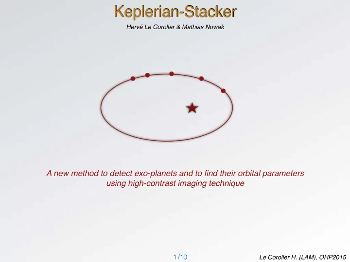
Keplerian-Stacker Herv Le Coroller & Mathias Nowak A new method - - PowerPoint PPT Presentation

Le Coroller H. (LAM), OHP2015

/10 1

Keplerian-Stacker

Hervé Le Coroller & Mathias Nowak

A new method to detect exo-planets and to find their orbital parameters using high-contrast imaging technique

/ 0 1

Le Coroller H. (LAM), OHP2015

Le Coroller H. (LAM), OHP2015

/10

Principle of the Coronagraphy

2 Telescope Mask Lyot Stop Coronagraphy image

With atmospheric turbulence

CCD

With atmospheric turbulence + AO correction

Phase masks generated by LAM/ONERA code (Fusco et al Optics Express 14, 7515-7534,2006)

Le Coroller H. (LAM), OHP2015

/10

Limitation due to quasi-static speckles

3 Simulation of SPHERE/IRDIS images r0=0.8 arcseconde 100 exposures of few millisecondes (frozen atmosphere) ⋋=1.6μm The static defaults follow an 1/f^2 law σ_mirror = 30 nm

Mathias Nowak simulations

800 mas 800 mas

Le Coroller H. (LAM), OHP2015

/10

Gain of 102-103 with ADI method (Marois, C. et al. 2006) to remove the quasi-static speckles

4 RAW IRDIS image t = 32s Filter obs = DBH23 cADI Reduced with the DC and

• R. Galicher software

Background 10 -3

!

Background 10 -5

!

Le Coroller H. (LAM), OHP2015

/10 5

K-Stacker principle

Le Coroller H. (LAM), OHP2015

/10 6

+ +

Center Star Planet E θ 2a X Y 2a(1-e2)1/2 Perihelion Aphelion

E(t) − esin[E(t)] =

• GM∗

a3 (t − t0)

7 parameters to describe the orbit: e = eccentricity [0-1] t0 = time at the perihelion passage a = semi-major axis θ0 = argument of periapsis 2 Euler angles (Omega=i=0 to begin) M* = Star Mass

E N

θ0

Earth

Equation of the Keplerien motion :

Transendante equation resolved by a Newton-Krylov method

K-Stacker principle

Le Coroller H. (LAM), OHP2015

/10

K-Stacker principle

7

An optimization Methode to Maximize:

X S(t0, e, a, θ0, Ω, i, M∗) = Pn

i=1 Fi

pPn

i=1 σ2 i

t0 t1 t2 t3 t1 t2 t3 t1 t2 t3 t1 t2 t3 t1 t2 t3

Le Coroller H. (LAM), OHP2015

/10 8

Nowak, M. & Le Coroller, H.,A&A, in preparation

S/N=8

Input

a = 5.24 ua e = 0.25 t0 = -2.13 years θ0 = -6.66 rad

Output

K-Stacker

Brute-Force + Gradiant

a (Semi-major axis) = 5.27 ua e (eccentricity) = 0.248 t0 (Perihelion time) = -2.07 years θ0 (Argument of periapsis) = -6.608 rad i = 0 Ω = 0 d = 10 pc M = 1M⊙

Observation conditions r0=0.8 arcsec; mR=8 100 images regularly spaced on 3 years S/N≃0.8 in each image

λ = 1.6µm

Le Coroller H. (LAM), OHP2015

/10 9

Input

a = 6.59 au e = 0.05 t0 = -0.9 years θ0 = 1.66 rad i=1.06 rad Ω= 1.18 rad

Output

K-Stacker

Brute-Force + Gradiant

a (Semi-major axis) = 6.80 au e (eccentricity) = 0.06 t0 (Perihelion time) = 0.89 year θ0 (Argument of periapsis) = 1.63 rad i = 1.07 rad Ω = 1.92 rad d = 10 pc M = 1M⊙

S/N=10

Observation conditions r0=0.8 arcsec; mR=8 25 images regularly spaced on 3 years S/N≃2.2 in each image

λ = 1.6µm

Nowak, M. & Le Coroller, H.,A&A, in preparation

Le Coroller H. (LAM), OHP2015

/10

K-Stacker: conclusion and perspectives

10

• 1) We have been able to detect planets at S/N total > 5 with

S/N<1 on individual frames !

• 3) K-Stacker should allow to detect fainter planets than with ADI observations only,

by integrating on longer time : 10^-8 with SPHERE

• 2) K-Stacker should work on ADI images.
• 4) Should help to optimize the observing strategy:

The K-Stacker method could be used to minimize the time that we should spend

• n each star to detect planets and its orbital parameters

Ex: If 1h of ADI observation allows to detect a planet at S/N=10, a K-Stacker observation of 6x10 min (ADI) spread over several months will allow to detect the same planet at the same S/N=10 level but will provide the

• rbital parameters !

accuracy on the planet position = 0.1 pixel on individual images of S/N<1 !!!

Le Coroller H. (LAM), OHP2015

/10 11

Le Coroller H. (LAM), OHP2015

/10

Amplitude of the planets motion in FWHM Airy disk

12

Le Coroller H. (LAM), OHP2015

/10 13

25 images réparties régulièrement sur 3 ans Seeing de 0.8’’, étoile guide de mag 8 (R) Planète à SNR=2.0 dans chaque image, injectée sur une orbite au hasard (6 paramètres), avec restriction des intervalles On ne s’intéresse qu’à la zone corrigée Paramètres de l’algorithme : Paramètre Valeur min Valeur max Nombre de points a 4 ua 7.5 ua 10 e 0.6 8 t0

• 1 ans

1 ans 10 i 0 rad 2.0 rad 12 Ω 0 rad 2.0 rad 5 θ0 0 rad 2.0 rad 12 Total de 576 000 orbites a essayer Les 20 meilleures sont retenues, et reoptimisées (BFGS, descente en gradient sous contraintes)

Pr Premiers ré résultat ats de de K-St Stack cker

• M. Nowak, 24 septembre 2015, ISAE Supaéro, Tou
• M. Nowak, H. Le Coroller, et al. (in prep)

a (ua) e t0 (an) Ω (rad) i (rad) θ0 (rad) Orbite réelle 6.80 0.06 0.89 1.92 1.07 1.63 Orbite trouvée 6.59 0.05

• 0.90

1.18 1.06 1.66

• Calcul executé en 10 h environ sur 1 processeur. Extrapolation : 3000 heures pour le cas non restreint

Avec 20 cœurs de 16 processeurs chacun (LAM) : une dizaine d’heures

• M. Nowak, 24 septembre 2015, ISAE Supaéro, Toulouse

16 12

Le Coroller H. (LAM), OHP2015

/10 14

Recherche par force brute (on essaie « toutes les possibilités ») combinée avec une méthode de descente en gradient Grille d’échantillonage force brute déterminée empiriquement (à partir de la largeur attendue du maximum) 108 possibilités environ Les quelques meilleures solutions de la grille sont réoptimisées avec une descente en gradient

L’algorithme

• M. Nowak, 24 septembre 2015, ISAE Supaéro, Toulouse

Le Coroller H. (LAM), OHP2015

/10 15 S’il n’y a pas de planète, la sommation correspond à une sommation au hasard : 𝑇𝑂𝑆 = 𝑂(0, 𝜏𝑗) 𝜏𝑗2 = 𝑂(0,1) Si l’orbite tombe sur celle d’une planète : 𝑇𝑂𝑆 = 𝑂 0, 1 + 𝑜×𝑇𝑞

𝜏𝑗2

On s’attend donc a des fluctuations d′écart type 1, et à la présence d’un pic détectable si 𝑇𝑞 > 5 𝜏/ 𝑜

• M. Nowak, 24 septembre 2015, ISAE Supaéro, Toulouse

Le Coroller H. (LAM), OHP2015

/10

Optimization using a Simulated annealing algorithm

16 Simulation Mathias Nowak Orbital parameters: 3 years of observation(Full orbit : 11.2 years). a=5; e=0.2 ; t0=3 years M=1M distance = 10Pc

⊙

Observation conditions: r0=0.8 arcsec mR=8 (étoile guide pour OA) Wind speed =10-15 m/s

λ = 1.6µm

S/N per image 1.5

! Solution found:

Le Coroller H. (LAM), OHP2015

/10

Recombined image by rotation and translation along the perihelion axis

17 S/N total= 17 Simulation Mathias Nowak

Le Coroller H. (LAM), OHP2015

/10 18

Dans le plan orbital : 2 paramètres (a, et e) 3 angles d’Euler pour positionner le plan orbital par rapport au plan du ciel (référence) : i, Ω, θ0 1 paramètre pour la position initiale : t0 2 paramètres supposés connus : masse et distance de l’étoile