Inverse Matrix Definition 1 0 . . . 0 0 1 . . . 0 - - PowerPoint PPT Presentation

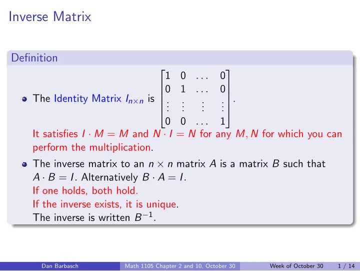
Inverse Matrix

Definition

The Identity Matrix In×n is      1 . . . 1 . . . . . . . . . . . . . . . . . . 1     . It satisfies I · M = M and N · I = N for any M, N for which you can perform the multiplication. The inverse matrix to an n × n matrix A is a matrix B such that A · B = I. Alternatively B · A = I. If one holds, both hold. If the inverse exists, it is unique. The inverse is written B−1.

Dan Barbasch Math 1105 Chapter 2 and 10, October 30 Week of October 30 1 / 14

Example of Inverse

A =   1 2 2 1 3 1   B =   2 4 6 −1 −4 −3 1 −1  . Find its inverse if it exists.

Dan Barbasch Math 1105 Chapter 2 and 10, October 30 Week of October 30 2 / 14

Encoding

Encode the message To be or not to be. In numbers, 20, 15, 27, 2, 5, 27, 15, 18, 27, 14, 15, 20, 27, 20, 15, 27, 2, 5. A to Z are 1 to 26 and spaces are 27. You substitute, and break up into 3 × 1 column vectors. The encoded message is B · vi. To decode, you break up into groups of three and make column vectors. Then apply B−1. B =   2 4 6 −1 −4 −3 1 −1  . ABCDEFGHIJ K L M N O P Q R S T U V W X 12345678910 11 12 13 14 15 16 17 18 19 20 21 22 23 24

Dan Barbasch Math 1105 Chapter 2 and 10, October 30 Week of October 30 3 / 14

Markov Chains

Transition Matrix P = (pij) where pij = P(j | i). Defining Properties: 0 ≤ pij ≤ 1,

j pij = 1.

Regular Pn for some n > 0 has positive entries only. Main Property: An equilibrium/fixed vector exists and is

• unique. v · P = v where v is a probability row vector.

Absorbing There is an i such that pii = 1. If so, all OTHER entries in row i are 0; pij = 0 for j = i. Also there is a positive probability to go from any state to an absorbing state. Main Property: Long Term Trend.

Dan Barbasch Math 1105 Chapter 2 and 10, October 30 Week of October 30 4 / 14

Examples

1

1 0.5 0.5

• 2

    0.4 0.3 0.3 0.3 0.7 0.2 0.2 0.3 0.3 0.6 0.4    

3

0.2 0.8 0.5 0.5

• 4

1 1

• 5

  0.2 0.8 0.8 0.2 0.8 0.2  

6

  1 1 1  

Dan Barbasch Math 1105 Chapter 2 and 10, October 30 Week of October 30 5 / 14

Example Continued

For (5), P2 =   0.68 0.16 0.16 0.16 0.68 0.16 0.16 .16 0.68   . So the matrix is regular.

Dan Barbasch Math 1105 Chapter 2 and 10, October 30 Week of October 30 6 / 14

Application

Example (Problem 25, Section 10.2)

The probability that a complex assembly line works correctly depends only

• n whether the line worked the last time it was used. There is a 0.9

chance that the line will work correctly if it worked correctly the last time, and a 0.8 chance that it will work correctly if it failed last time. Set up a transition matrix, and find the long range probability that the line will work correctly.

Dan Barbasch Math 1105 Chapter 2 and 10, October 30 Week of October 30 7 / 14

Answer.

The matrix is 0.9 0.1 0.8 0.2

• . This is regular. We need to solve the system
• x,

y

• ·

0.9, 0.1 0.8, 0.2

• =
• x,

y

• .

This is

• 0.9x + 0.8y,

0.1x + 0.2y

• =
• x,

y

• We can rewrite it as
• −0.1x + 0.8y

= 0 0.1x − 0.8y = 0. The two equations are x = 8y. So the equilibrium vector is

• 8/9

1/9

• .

In general, the coefficient matrix of the system is PT − I, and you set every equation equal to 0: [PT − I | 0]. Transpose means that you interchange rows and columns.

Dan Barbasch Math 1105 Chapter 2 and 10, October 30 Week of October 30 8 / 14

Regular Markov Chains, Summary

1 The matrix P has positive entries only. 2 There is a unique equilibrium (probability) vector V such that

V · P = V .

3 limm→∞ Pm =

   V1 . . . Vn . . . . . . . . . V1 . . . Vn    , limm→∞ v · Pm = V .

4 To solve for V , you need to solve the system [Pt − In×n | 0]. There is

a unique solution satisfying 0 ≤ Vj ≤ 1 and V1 + · · · + Vn = 1.

Dan Barbasch Math 1105 Chapter 2 and 10, October 30 Week of October 30 9 / 14

Previous Example

  −0.1 0.8 0.1 −0.8 1 1 1   →   1 −8 1 1 1   → −9 −1 1 1 1

• →

1 1/9 1 1 1

• →

→ 1 1/9 1 8/9

• →

1 8/9 1 1/9

• Dan Barbasch

Math 1105 Chapter 2 and 10, October 30 Week of October 30 10 / 14

Absorbing Markov Chains

1 The matrix P has some pii = 1. You rearrange the states so that the

matrix is P = I R Q

• . For each state there must a positive

probability for it to go to an equilibrium state. This means each row

• f F moust have a nonzero entry.

2 limm→∞ Pm =

• I

(I − Q)−1R

• . The rows of (I − Q)−1R tell you

the probabilities of ending up in the state corresponding to the

• column. The matrix F = (I − Q)−1 is called the fundamental matrix.

The number fij give the number of visits to state j before being absorbed, given that the current state is i.

Dan Barbasch Math 1105 Chapter 2 and 10, October 30 Week of October 30 11 / 14

Gambler’s Ruin

Two players A and B, play a game. They toss a coin. If heads, then A pays B $1. If tails, B pays A $1. They start out with a total of $3. The game ends whenever on of the players is broke. Analyze the game.

Dan Barbasch Math 1105 Chapter 2 and 10, October 30 Week of October 30 12 / 14

Classification of States I

Question: How to tell if a Markov Chain is regular.

1 We say j is accessible from i if pm(i, j) > 0 for some m > 0. i, j

communicate, i ≃ j, if pn(i, j) > 0 and pm(j, i) > 0 for some m, n > 0.

2 i ≃ i 3 i ≃ j implies j ≃ i 4 i ≃ j and j ≃ k implies i ≃ j 5 The sets of equivalent states are called classes 6 A Markov Chain is irreducible if all states are in a single class. 7 Regular implies irreducible. 8 Absorbing states are single classes. 9 i is called transient if fi = P(i for some m | i) = 1. 10 i is called recurrent if fi = P(i for some m | i) < 1. Dan Barbasch Math 1105 Chapter 2 and 10, October 30 Week of October 30 13 / 14

Classification of States II

To find the equivalence classes:

1 Draw the states 2 Forget the probabilities on the diagonal 3 Join two states by an edge if p(i, j) > 0 and p(j, i) > 0. 4 If only one is > 0, draw an arrow. Dan Barbasch Math 1105 Chapter 2 and 10, October 30 Week of October 30 14 / 14