
SLIDE 1
Introduction to Machine Learning ML-Basics: Losses & Risk - - PowerPoint PPT Presentation
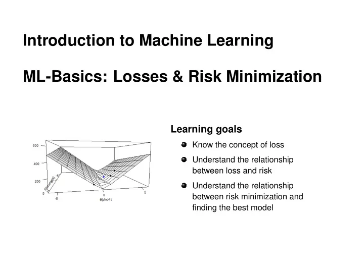
Introduction to Machine Learning ML-Basics: Losses & Risk Minimization Learning goals Know the concept of loss Understand the relationship between loss and risk Understand the relationship between risk minimization and finding the best
c
c
c
c
n
c
n
n does not make a difference in optimization, so we will
n
c
c
c