Introduction to Graphs nodes. edges between pairs of nodes. - - PowerPoint PPT Presentation

Introduction to Graphs

Tyler Moore

CSE 3353, SMU, Dallas, TX

Lecture 5

Some slides created by or adapted from Dr. Kevin Wayne. For more information see http://www.cs.princeton.edu/~wayne/kleinberg-tardos

3

• Notation.

nodes. edges between pairs of nodes. Captures pairwise relationship between objects. Graph size parameters: .

• 2 / 24

4

• 3 / 24

5

• 4 / 24

6

• Figure 1. Largest Connected Subcomponent of the Social N etwork in the Framingham H eart Study in the Year 2000.

Each circle (node) represents one person in the data set. There are 2200 persons in this subcomponent of the social

• network. Circles with red borders denote women, and circles with blue borders denote men. The size of each circle

is proportional to the person’s body-mass index. The interior color of the circles indicates the person’s obesity status: yellow denotes an obese person (body-mass index, ≥30) and green denotes a nonobese person. The colors of the ties between the nodes indicate the relationship between them: purple denotes a friendship or marital tie and orange denotes a familial tie.

5 / 24

Social Network as a Graph

Alice Bob Charlie Dawn Eve Fred George Nodes: people Edges: friendship

6 / 24

Road Network as a Graph

Main St 1st Ave 2nd Ave 3rd Ave Main St Elm St Aspen Ave 5th Ave Park St Main St 5th Ave

Nodes: intersections Edges: roads

7 / 24

Electronic Circuits as a Graph

B 20Ω 10Ω vx

S 5 vx

5Ω A Vertices: junctions Edges: components

8 / 24

Course Dependencies as a Graph

CSE1341 CSE1342 CSE2353 CSE2341 CSE3353 CSE5338 Nodes: courses Edges: prerequisites

10 / 24

Maze as a Graph

Nodes: rooms; edges: doorways

11 / 24

Flavors of Graphs

The first step in any graph problem is recognizing that you have a graph problem It’s not always obvious! The second step in any graph problem is determining which flavor of graph you are dealing with Learning to talk the talk is an important part of walking the walk The flavor of graph has a big impact on which algorithms are appropriate and efficient

12 / 24

Directed vs. Undirected Graphs

A B C D E F G Undirected A B C D E F G Directed A graph G = (V , E) is undirected if edge (x, y) ∈ E implies that (y, x) is also in E Road networks between cities are typically undirected Street networks within cities are almost always directed because of

• ne-way streets

What about online social networks?

13 / 24

7

• graph

node edge communication telephone, computer fiber optic cable circuit gate, register, processor wire mechanical joint rod, beam, spring financial stock, currency transactions transportation street intersection, airport highway, airway route internet class C network connection game board position legal move social relationship person, actor friendship, movie cast neural network neuron synapse protein network protein protein-protein interaction molecule atom bond 13 / 24

39

• directed graph

node directed edge transportation street intersection

• ne-way street

web web page hyperlink food web species predator-prey relationship WordNet synset hypernym scheduling task precedence constraint financial bank transaction cell phone person placed call infectious disease person infection game board position legal move citation journal article citation

• bject graph
• bject

pointer inheritance hierarchy class inherits from control flow code block jump 14 / 24

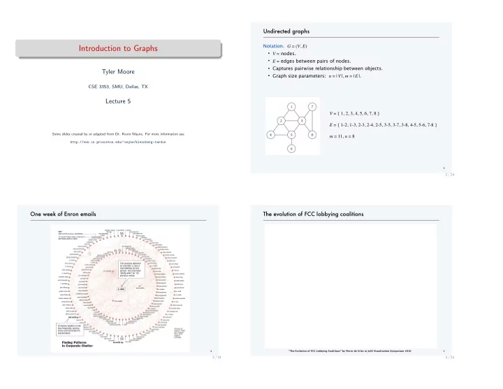
Weighted vs. Unweighted Graphs

A B C D E F G Unweighted A B C D E F G

10 4 1 7 5 8 19 4 10 6 8

Weighted In weighted graphs, each edge (or vertex) of G is assigned a numerical value, or weight The edges of a road network graph might be weighted with their length, drive-time or speed limit In unweighted graphs, there is no cost distinction between various edges and vertices

15 / 24

Simple vs. Non-simple Graphs

A B C D E F G Simple A B C D E F G Non-simple Certain types of edges complicate the task of working with graphs. A self-loop is an edge (x, x) involving only one vertex. An edge (x, y) is a multi-edge if it occurs more than once in the graph. Any graph without self-loops and multi-edges is called simple. Which of the earlier example graphs can be non-simple?

16 / 24

Sparse vs. Dense Graphs

A B C D E F G Sparse A B C D E F G Dense Graphs are sparse when only a small fraction of the possible number

• f vertex pairs actually have edges defined between them.

Graphs are usually sparse due to application-specific constraints Road networks must be sparse because of road junctions Typically dense graphs have a quadratic number of edges while sparse graphs are linear in size

17 / 24

Cyclic vs. Acyclic Graphs

A B C D F G Cyclic A B C D F G Acyclic An acyclic graph does not contain any cycles Trees are connected, acyclic, undirected graphs Directed acyclic graphs are called DAGs DAGs arise naturally in scheduling problems, where a directed edge (x, y) indicates that x must occur before y.

18 / 24

Labeled vs. Unlabeled Graphs

A B C D E F G Labeled Unlabeled In labeled graphs, each vertex is assigned a unique name or identifier to distinguish it from all other vertices. An important graph problem is isomorphism testing: determining whether the topological structure of two graphs are in fact identical if we ignore any labels.

19 / 24

More Graph Terminology

A path is a sequence of edges connecting two vertices Two common problems: (1) does a path exist between A and B? (2) what is the shortest path between A and B? A graph is connected if there is a path between any two vertices A directed graph is strongly connected if there is a directed path between any two vertices. The degree of a vertex is the number of edges adjacent to it

20 / 24

8

• Adjacency matrix. -by- matrix with if is an edge.

Two representations of each edge. Space proportional to . Checking if is an edge takes Θ time. Identifying all edges takes Θ time.

1 2 3 4 5 6 7 8 1 0 1 1 0 0 0 0 0 2 1 0 1 1 1 0 0 0 3 1 1 0 0 1 0 1 1 4 0 1 0 0 1 0 0 0 5 0 1 1 1 0 1 0 0 6 0 0 0 0 1 0 0 0 7 0 0 1 0 0 0 0 1 8 0 0 1 0 0 0 1 0

21 / 24

9

• Adjacency lists. Node indexed array of lists.

Two representations of each edge. Space is Θ. Checking if is an edge takes time. Identifying all edges takes Θ time.

1 2 3 2 3 4 2 5 5 6 7 3 8 8 1 3 4 5 1 2 5 8 7 2 3 4 6 5 degree = number of neighbors of u 3 7

22 / 24

Graph Data Structures

a b d c e f h g Option 1: Adjacency Sets

a , b , c , d , e , f , g , h = range (8) N = [ {b , c , d , e , f } , # a {c , e } , # b {d } , # c {e } , # d { f } , # e {c , g , h } , # f { f , h } , # g { f , g} # h ] > > > b i n N[ a ] # Neighborhood membership True > > > l e n (N[ f ] ) # Degree 3

23 / 24

Graph Data Structures

a b d c e f h g Option 2: Adjacency Lists

a , b , c , d , e , f , g , h = range (8) N = [ [ b , c , d , e , f ] , # a [ c , e ] , # b [ d ] , # c [ e ] , # d [ f ] , # e [ c , g , h ] , # f [ f , h ] , # g [ f , g ] # h ] > > > b i n N[ a ] # Neighborhood membership True > > > l e n (N[ f ] ) # Degree 3

23 / 24

Graph Data Structures

a b d c e f h g

2 1 3 9 4 4 3 8 7 5 2 2 2 1 6 9 8

Option 3: Adjacency Dictionaries w/ Edge Weights

a , b , c , d , e , f , g , h = range (8) N = [ {b : 2 , c : 1 , d : 3 , e : 9 , f :4 } ,#a {c : 4 , e : 3 } , #b {d : 8} , #c {e : 7 } , #d { f : 5} , #e {c : 2 , g : 2 , h : 2} , #f { f : 1 , h : 6 } , #g { f : 9 , g :8} #h ] > > > b i n N[ a ] # Neighborhood membership True > > > l e n (N[ f ] ) # Degree 3 > > > N[ a ] [ b ] # Edge weight f o r ( a , b ) 2

23 / 24

Graph Data Structures

a b d c e f h g Option 4: Dictionaries w/ Adjacency Sets

N = { ’ a ’ : s e t ( ’ bcdef ’ ) , ’ b ’ : s e t ( ’ ce ’ ) , ’ c ’ : s e t ( ’ d ’ ) , ’ d ’ : s e t ( ’ e ’ ) , ’ e ’ : s e t ( ’ f ’ ) , ’ f ’ : s e t ( ’ cgh ’ ) , ’ g ’ : s e t ( ’ fh ’ ) , ’ h ’ : s e t ( ’ fg ’ ) } > > > ’ b ’ i n N[ ’ a ’ ] # Neighborhood membership True > > > l e n (N[ ’ f ’ ] ) # Degree 3

23 / 24

Graph Data Structures

a b d c e f h g Option 5: Adjacency Matrix (using nested lists)

a , b , c , d , e , f , g , h = range (8) # a b c d e f g h N = [ [ 0 , 1 , 1 , 1 , 1 , 1 , 0 , 0 ] , # a [ 0 , 0 , 1 , 0 , 1 , 0 , 0 , 0 ] , # b [ 0 , 0 , 0 , 1 , 0 , 0 , 0 , 0 ] , # c [ 0 , 0 , 0 , 0 , 1 , 0 , 0 , 0 ] , # d [ 0 , 0 , 0 , 0 , 0 , 1 , 0 , 0 ] , # e [ 0 , 0 , 1 , 0 , 0 , 0 , 1 , 1 ] , # f [ 0 , 0 , 0 , 0 , 0 , 1 , 0 , 1 ] , # g [ 0 , 0 , 0 , 0 , 0 , 1 , 1 , 0 ] ] # h > > > a , b , c , d , e , f , g , h = range (8) > > > N[ a ] [ b ] # Neighborhood membership 1 > > > sum(N[ f ] ) # Degree 3

23 / 24

Graph Data Structures

a b d c e f h g

2 1 3 9 4 4 3 8 7 5 2 2 2 1 6 9 8

Option 6: Weighted Adjacency Matrix (using nested lists)

a , b , c , d , e , f , g , h = range (8) = f l o a t ( ’ i n f ’ ) # a b c d e f g h W = [ [ 0 , 2 , 1 , 3 , 9 , 4 , , ] , # a [ , 0 , 4 , , 3 , , , ] , # b [ , , 0 , 8 , , , , ] , # c [ , , , 0 , 7 , , , ] , # d [ , , , , 0 , 5 , , ] , # e [ , , 2 , , , 0 , 2 , 2 ] , # f [ , , , , , 1 , 0 , 6 ] , # g [ , , , , , 9 , 8 , 0 ] ] # h > > > i n f = f l o a t ( ’ i n f ’ ) > > > W[ a ] [ b ] < i n f # Neighborhood membership True > > > W[ c ] [ e ] < i n f # Neighborhood membership F a l s e > > > sum(1 f o r w i n W[ a ] i f w < i n f ) − 1 # Degree 5

23 / 24

Trade-offs Between Adjacency Lists and Adjacency Matrices

When the text refers to adjacency lists, it means adjacency linked lists Adjacency linked lists use less memory for sparse graphs than matrices Finding vertex degree is Θ(1) vs. Θ(n) in matrices In Python, adjacency lists are technically adjacency dynamic arrays (respectively sets and dictionaries for other representations) Python adjacency lists/sets/dictionaries use less memory than adjacency matrices implemented in Python They are also Θ(1) to find vertex degree Within Python, adjacency sets offer expected Θ(1) membership checking vs. Θ(1) for lists For graph traversal, adjacency lists execute faster than sets.

24 / 24