Introduction to Credibility 1 Limited Fluctuation Example 1 - PDF document

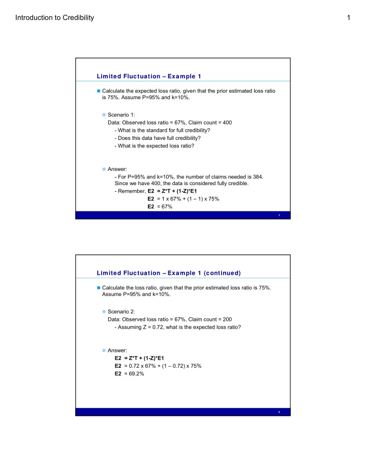
Introduction to Credibility 1 Limited Fluctuation – Example 1  Calculate the expected loss ratio, given that the prior estimated loss ratio is 75%. Assume P=95% and k=10%.  Scenario 1: Data: Observed loss ratio = 67%, Claim count = 400 - What is the standard for full credibility? - Does this data have full credibility? - What is the expected loss ratio?  Answer: - For P=95% and k=10%, the number of claims needed is 384. Since we have 400, the data is considered fully credible. - Remember, E2 = Z*T + (1-Z)*E1 E2 = 1 x 67% + (1 – 1) x 75% E2 = 67% 1 Limited Fluctuation – Example 1 (continued)  Calculate the loss ratio, given that the prior estimated loss ratio is 75%. Assume P=95% and k=10%.  Scenario 2: Data: Observed loss ratio = 67%, Claim count = 200 - Assuming Z = 0.72, what is the expected loss ratio?  Answer: E2 = Z*T + (1-Z)*E1 E2 = 0.72 x 67% + (1 – 0.72) x 75% E2 = 69.2% 2

Introduction to Credibility 2 Limited Fluctuation – Example 1 (Revisited)  Calculate the loss ratio, given that the prior estimated loss ratio is 75%. Assume P=95% and k=10%.  Scenario 2: Data: Observed loss ratio = 67%, Claim count = 200  Answer: E2 = Z*T + (1-Z)*E1 E2 = √ (200/384) x 67% + (1 – √ (200/384)) x 75% E2 = 69.2% 3 Limited Fluctuation – Example 2  For the 3 and 5-year periods, calculate the credibility (using the square root rule), credibility-weighted loss ratio and indicated change, given that the expected loss ratio is 75%. Assume P= 90% and k = 2.5%. Loss Claim Year Ratio Count 2007 67% 530 2008 77% 610 2009 79% 630 79.0% = 81% x (0.67) + 2010 77% 620 75% x (1 - 0.67) 2011 86% 690 Cred-Wght Indicated Credibility Loss Ratio Rate Chg '09-'11 81% 1,940 67% 79.0% 5.3% '07-'11 77% 3,080 84% 76.7% 2.3% 67%= √ (1940/4326 ) 5.3% = 79.0%/75.0% 4

Introduction to Credibility 3 Limited Fluctuation – Example 3  Given a current territory factor of 1.08, determine the indicated territory factor with 5 years of data. The frequency distribution is Poisson and the severity coefficient of variation of 1.5. Use the square root rule and the limited fluctuation formula for pure premium. Assume that you want to be within 5% of the true value 90% of the time. The statewide frequency is 0.20 and fixed expenses are 15%. Territory Territory Territory Statewide Year Exposure Claim Count Loss Ratio Loss Ratio 2006 3,000 330 125% 78% 2007 3,020 420 153% 83% 2008 3,030 630 269% 85% 2009 3,020 210 122% 79% 2010 3,050 190 108% 72% '06-'10 15,120 1,780 162% 80% 5 Limited Fluctuation – Example 3 (continued) N = (z p / k) 2 * (Var(N)/E(N) + Var(S)/E(S) 2 )  If we want to be within 5% of the true value 90% of the time, (z p / k) 2 is 1,082.  Remember, with a Poisson distribution, Var(N) = E(N), the second term is 1. The third term is the square of the coefficient of variation, which is 1.5 2 . N claims = 1,082 * ( 1 + 1.5 2 ) = 3,516.5  Given the 5-year statewide frequency of 0.2: N exposures = 3,516.5 / 0.2 = 17,582.5 6

Introduction to Credibility 4 Limited Fluctuation – Example 3 (continued)  To show the impact of our selection of an exposure standard instead of a claims standard. Territory Territory Exposure Claim Year Exposure Claim Count Credibility Credibility 2006 3,000 330 41.3% 30.6% 2007 3,020 420 41.4% 34.6% 2008 3,030 630 41.5% 42.3% 2009 3,020 210 41.4% 24.4% 2010 3,050 190 41.6% 23.2% '06-'10 15,120 1,780 92.7% 71.1% Using a claims standard of 3,517 and an exposure standard of 17,583 7 Limited Fluctuation – Example 3 (continued)  Determine what the indicated territorial factor, assuming 15% for fixed expenses. Territory Territory Statewide Cred Wght Year Loss Ratio Credibility Loss Ratio Loss Ratio '06-'10 162% 92.7% 80% 156.0% 156.0% = 92.7% x 162% + 7.3% x 80% The final indicated territorial factor is (156% / 80%)*0.85 + 0.15 = 1.81 An alternative approach would be to calculate the indicated factor prior to applying credibility, and then credibility weight the current factor with the indicated factor. 8

Introduction to Credibility 5 Least Squares – Example Assuming that you have the following book of business, calculate the EVPV,  VHM, K, and Z. The prior estimate of the frequency is 0.517. With 4 years of observations and an observed frequency of 0.75, what is the estimated future frequency? Assume the claims are binomially distributed. Risk P(Claim) P(Risk) Variance Mean 2 Low 40% 65% 0.24 0.16 Medium 70% 23% 0.21 0.49 High 80% 12% 0.16 0.64 Total 51.7% 100% 0.2235 0.2935  EVPV: For binomial, variance = P(claim) x P(no claim) = (40%)(60%)(65%) + (70%)(30%)(23%) + (80%)(20%)(12%) = 0.2235  VHM: Mean 2 – (Mean) 2 = 0.2935 – (0.517) 2 = 0.0262 9 Least Squares – Example (continued) To determine K, we use K = EVPV/VHM, which is  K = 0.2235 / 0.0262 = 8.53 Since we’re told that we have 4 years of observations, n = 4. Therefore,  Z = n / (n + K)  4 / (4 + 8.53) = 0.319. The prior estimate of frequency is the same as the mean calculated before,  0.517, and the observed data results in a frequency of 0.75. This observed data as 31.9% credibility, so… E2 = Z * T + (1 – Z) * E1  31.9% * 0.75 + 68.1% * 0.517 = 0.5913 10