Introduction: Mathematical optimization Motivating Example - - PowerPoint PPT Presentation

SLIDE 1

Introduction: Mathematical optimization

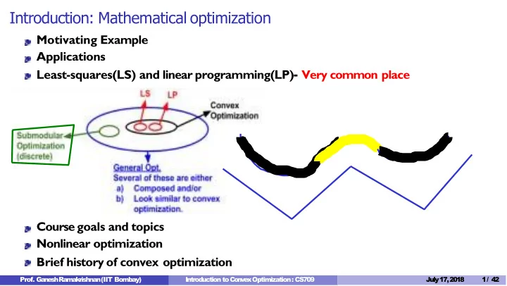
Motivating Example Applications Least-squares(LS) and linear programming(LP)- Very common place Course goals and topics Nonlinear optimization Brief history of convex optimization

• Prof. G

a n e s h Ramakrishnan (IIT Bombay) Introduction to C

• n

v e x Optimization : CS709 July 17,2018 1/ 42

SLIDE 2

Almost Every Problem can be posed as an Optimization Problem

G i v e n a s e t C⊆ ℜn find t h e ellipsoidE⊆ ℜ

n that i

s

• f s

m a l l e s t v

• l

u m e s u c hthatC⊆E. Hint: First work out the problem in lower dimensions

C x in C is a vector of size n x = [x1,x2......xn] Constraint: x1^2/a1^2 + x2^2/a2^2 + ....xn^2/an^2 <= 1 a2

• Prof. G

a n e s h Ramakrishnan (IIT Bombay) Introduction to C

• n

v e x Optimization : CS709 July 17,2018 4 / 42

a1 NEED A ROTATED+TRANSLATED VERSIO

SLIDE 3

Almost Every Problem can be posed as an Optimization Problem

G i v e n a s e t C⊆ ℜ

n find t

h e ellipsoidE⊆ ℜ

n that i

s

• f s

m a l l e s t v

• l

u m e s u c hthatC⊆E. Hint: First work out the problem in lower dimensions Sphere S

r ⊆ ℜ n c

e n t e r e d at0is e x p r e s s e da s :

Sr = { ||x||_2 <= r} 2-norm is the square root of sum of squares

• f the individual components of x
• Prof. G

a n e s h Ramakrishnan (IIT Bombay) Introduction to C

• n

v e x Optimization : CS709 July 17,2018 4 / 42

SLIDE 4

Almost Every Problem can be posed as an Optimization Problem

u A' mxn n m Our basic ellipsoid had A' = diagonal

G i v e n a s e t C⊆ ℜ

n find t

h e ellipsoidE⊆ ℜ

n that i

s

• f s

m a l l e s t v

• l

u m e s u c hthatC⊆E. Hint: First work out the problem in lower dimensions Sphere S

r ⊆ ℜ n c

e n t e r e d at0is e x p r e s s e d as:S

r ={u∈ ℜ n|∥u∥2 ≤r}

EllipsoidE⊆ ℜ

n i

s e x p r e s s e da s :

Av + b A'u + b' Ellipsoid is a rotated, scaled and translated version of the sphere

• Prof. G

a n e s h Ramakrishnan (IIT Bombay) Introduction to C

• n

v e x Optimization : CS709 July 17,2018 4 / 42

SLIDE 5

Almost Every Problem can be posed as an Optimization Problem

G i v e n a s e t C⊆ ℜ

n find t

h e ellipsoidE⊆ ℜ

n that i

s

• f s

m a l l e s t v

• l

u m e s u c hthatC⊆E. Hint: First work out the problem in lower dimensions Sphere S

r ⊆ ℜ n c

e n t e r e d at0is e x p r e s s e d as:S

r ={u∈ ℜ n|∥u∥2 ≤r}

EllipsoidE⊆ ℜ

n i

s e x p r e s s e da s :

n

E= v∈ ℜ|Av+b∈S

1

{ } {

n 2

= v∈ ℜ |∥Av+b∥ ≤ }

n ++

1 . Here,A∈S , that is,Ais ann×n(strictly) p

• s

it iv e definitematrix. The optimization p r

• b

l e m willbe:

1) A is an nxn matrix (Sphere and Ellipsoid are both in R^n) 2) This brings an additional constraint that A is symmetic, and it is positive definite

• Prof. G

a n e s h Ramakrishnan (IIT Bombay) Introduction to C

• n

v e x Optimization : CS709 July 17,2018 4 / 42

3)That is, A has positive eigen values.. 4) The positive eigenvalues will correspond to scaling of the axis and corresponding eigenvectors to the new axes 5) The volume is proportional tothe product of lengths of eigenvalues

SLIDE 6

Almost Every Problem can be posed as an Optimization Problem

G i v e n a s e t C⊆ ℜ

n find t

h e ellipsoidE⊆ ℜ

n that i

s

• f s

m a l l e s t v

• l

u m e s u c hthatC⊆E. Hint: First work out the problem in lower dimensions Sphere S

r ⊆ ℜ n c

e n t e r e d at0is e x p r e s s e d as:S

r ={u∈ ℜ n|∥u∥2 ≤r}

EllipsoidE⊆ ℜ

n i

s e x p r e s s e da s :

n

E= v∈ ℜ|Av+b∈S

1

{ } {

n

= v∈ ℜ|∥Av+b∥

2

} ≤1 . Here,A

n ++

∈S , that is,Ais ann×n(strictly) p

• s

it iv e definite matrix. The

• ptimization p

r

• b

l e m willbe: m in im i z e

[a11,a12..,ann,b1,..bn]

det(A−1) s u b j e c ttov

July 17,2018 4 / 42

TAv>0,∀v̸= 0

A is positive definite

∥Av+b∥ 2 ≤1,∀v∈C

C is contained in the Ellipsoid C Can forall v be changed to checking for a finite n u

P r

m

• f

. G

b

a n

e

e s

r

hR

• a

m

f

a k

b

r i s h

• n

a

u

nn ( I I Td Ba

• mr

by a y )points I n? t r

• d

u c t i

• n

to C

• n

v e x Optimization : CS709

SLIDE 7

Almost Every Problem can be posed as an Optimization Problem (contd.)

Give n a polygonP⊆ ℜ

n

find t h e ellipsoidE⊆ ℜ

n that i

s

• f s

m a l l e s t v

• l

u m e s u c hthat e t v1,v 2, ...vp b e t h e c

• r

n e r s

• f t

h epolygonP P⊆E. L The

• ptimization p

r

• b

l e m willbe: m in im i z e

[a11,a12..,ann,b1,..bn]

s u b j e c tto−v

i

det(A−1)

TAv>0,∀v̸= 0

∥Av +b∥ 2 ≤1,i∈{1..p}

Introduction to C

• n

v e x Optimization: CS709 July 17, 2018 5 / 42

v1 v2 v3 v4 v5 Given that the specified set S is indeed a polygon, is this problem with a simplified set of constraints equivalent to the original problem?

P r

Y

• f

.

E

G

S

a n e s hRamakrishnan (IIT Bombay)

SLIDE 8

Almost Every Problem can be posed as an Optimization Problem (contd.)

G i v e n a polygonP⊆ ℜ

n find t

h e ellipsoidE⊆ ℜ

n that i

s

• f s

m a l l e s t v

• l

u m e s u c hthat P⊆E. L e t v1,v 2, ...vp b e t h e c

• r

n e r s

• f t

h e polygonP The

• ptimization p

r

• b

l e m willbe: m in im i z e

[a11,a12..,ann,b1,..bn]

s u b j e c tto−v det(A−1)

TAv>0,∀v̸= 0

∥Avi +b∥ 2 ≤1,i∈{1..p} H

• w

w

• u

l d y

• u

p

• s

e a n

• ptimization

p r

• b

l e m to find t h e ellipsoidE ′ of l a r g e s t v

• l

u m e that fitsi n s i d e C ?

• Prof. G

a n e s h Ramakrishnan (IIT Bombay) Introduction to C

• n

v e x Optimization : CS709 July 17,2018 5 / 42

SLIDE 9

So Again: Mathematical optimization

fi :ℜ

n→ℜ,i= 1, ...,m: c

• n

s t r a in tfu n c t io n s m i n i

x

m i z e f0(x) s u b j e c t tof i(x)≤b i,i= 1, . . . ,m. x= (x 1, ...,x n): optimizationv a r i a b l e s

• ptimal solutionx ∗

h a s s m a l l e s t v a l u e

• ff

0 a

m

• n

g all v e c t

• r

s that s a t is fy t h ec

• n

s t r a i n t s

• Prof. G

a n e s h Ramakrishnan (IIT Bombay) Introduction to C

• n

v e x Optimization : CS709 July 17,2018 6 / 42

SLIDE 10

Examples

portfolio optimization v a r ia b le s : a m

• u

n t s i n v e s t e d in differenta s s e t s c

• n

s t r a in t s : budget, max./min. i n v e s t m e n t p e r a s s e t ,m i n i m u m return

• b

je c t iv e : o v e r a ll r is k

• r

returnv a r i a n c e

• Prof. G

a n e s h Ramakrishnan (IIT Bombay) Introduction to C

• n

v e x Optimization : CS709 July 17,2018 7 / 42

SLIDE 11

Examples

Data fitting- Machine learning v a r ia b le s : m

• d

e lp a r a m e t e r s c

• n

s t r a in t s : prior information, p a r a m e t e r limits

• b

je c t iv e : m e a s u r e

• f misfit o

r p r e d ic t io ne r r

• r
• Prof. G

a n e s h Ramakrishnan (IIT Bombay) Introduction to C

• n

v e x Optimization : CS709 July 17,2018 9 / 42

SLIDE 12

Applications

S p a m De t e c t io n Digit Re c

• g

n it io n M e d ic a ld i a g n

• s

i s Bio-diversity c l a s s i f i c a t i

• n

Buying

• r

s e llin gp r

• d

u c t s

• Prof. G

a n e s h Ramakrishnan (IIT Bombay) Introduction to C

• n

v e x Optimization : CS709 July 17,2018 12 / 42

SLIDE 13

Problem in Perspective

1,c 2,...,c k}

G i v e n d a t a pointsx

i,i= 1,2, . . . ,m

P

• s

s i b l e c l a s s c h

• i

c e s : c 1,c 2, . . . ,c k Wish to g e n e r a t e amapping/classifier f:x→{ c T

• g

e t c l a s slabelsy1,y 2,...,y m

• Prof. G

a n e s h Ramakrishnan (IIT Bombay) Introduction to C

• n

v e x Optimization : CS709 July 17,2018 13 / 42

SLIDE 14

Problem in Perspective

In g e n e r a l, s e r i e s

• fm

a p p i n g s x f(·)

g(· ) h(· ) 1 2

−→y −→z −→{c ,c , . . .,

k

c }

eg: neural networks

• Prof. G

a n e s h Ramakrishnan (IIT Bombay) Introduction to C

• n

v e x Optimization : CS709 July 17,2018 14 / 42

SLIDE 15

Problem in Perspective

In g e n e r a l, s e r i e s

• fm

a p p i n g s x f(·)

g(· )

−→y −→

h(· )

z −→{c ,

1 2 k

c ,...,c } wh e re y ,za r e in s

• m

e latents p a c e .

• Prof. G

a n e s h Ramakrishnan (IIT Bombay) Introduction to C

• n

v e x Optimization : CS709 July 17,2018 14 / 42

SLIDE 16

Perceptron Classifier

C

• n

s i d e r ab in a r y c l a s s i f i c a t i

• nproblem:f(x)∈{−1,+1}

w^Tx + b w

Objective: L e a r n a lin e a r c l a s s i f i e r With linearlys e p a r a b ilit y

Extent of misclassification of apoint is = -y(w^Tx + b)

• Prof. G

a n e s h Ramakrishnan (IIT Bombay) Introduction to C

• n

v e x Optimization : CS709 July 17,2018 16 / 42

SLIDE 17

Perceptron Classifier

C

• n

s i d e r ab in a r y c l a s s i f i c a t i

• nproblem:f(x)∈{−1,+1}

Objective: L e a r n alin e a rc l a s s i f i e r With linearly separabilit y, a n y finite t i m e le a r n in galgorithm ?

• Prof. G

a n e s h Ramakrishnan (IIT Bombay) Introduction to C

• n

v e x Optimization : CS709 July 17,2018 16 / 42

SLIDE 18

Perceptron Classifier

C

• n

s i d e r ab in a r y c l a s s i f i c a t i

• nproblem:f(x)∈{−1,+1}

Desirable: Any n e w input pattern s im ila r to a s e e n patternisclassifiedcorrectly L i n e a r Cla s s ific a t io n ?

w⊤ϕ(x) +b≥0for +ve points (y= +1) w⊤ϕ(x) +b<0for -ve points (y= -1) w,ϕ∈IR m

• Prof. G

a n e s h Ramakrishnan (IIT Bombay) Introduction to C

• n

v e x Optimization : CS709 July 17,2018 17 / 42

SLIDE 19

• Prof. G

a n e s h Ramakrishnan (IIT Bombay) Introduction to C

• n

v e x Optimization : CS709 July 17,2018 20 / 42

SLIDE 20

Perceptron Update Rule: Error Perspective

U n s i g n e d d i s t a n c e from hyperplane:yw T(ϕ(x)) wTϕ(x) = 0 b ϕ(x0) ϕ(x) D w

Negative of the unsigned distance is the error

• Prof. G

a n e s h Ramakrishnan (IIT Bombay) Introduction to C

• n

v e x Optimization : CS709 July 17,2018 24 / 42

SLIDE 21

Perceptron Update Rule: Error Minimization

P e r c e p t ro n u p d a t e t r ie s to m in im i z e t h e e r r

• rfunction

E= n e g a t i v e

• f s

u m

• f u

n s i g n e d d i s t a n c e s

• v

e r m i s c l a s s i f i e d e x a m p l e s = s u m

• f

m i s c l a s s i f i c a t i

• nc
• s

t s ∑ E=− ywTϕ(x)

(x,y)∈M

whereM⊆Dis t h e s e t

• f m

i s c l a s s i f i e de x a m p l e s .

• Prof. G

a n e s h Ramakrishnan (IIT Bombay) Introduction to C

• n

v e x Optimization : CS709 July 17,2018 25 / 42

SLIDE 22

Machine Learning as Optimization

w∗ a r g m i n L(w) +Ω(∥w∥ 2) b =

w

(1)

0-1 Loss:

L(w) = ∑

(x,y) δ (y̸=w Tϕ(x))

(2)

Minimizing t h e 0-1 L

• s

s i s NP-hard. W e t h e r e f

• r

e lo

• k

fors u r r

• g

a t e s . Perceptron:A N

• n
• c
• n

v e xS u r r

• g

a t e

L(w) =− ∑

(x,y)∈M ywTϕ(x)

(3)

whereM⊆Dis t h e s e t

• f m

i s c l a s s i f i e de x a m p l e s .

• Prof. G

a n e s h Ramakrishnan (IIT Bombay) Introduction to C

• n

v e x Optimization : CS709 July 17,2018 26 / 42

SLIDE 23

Convex Surrogates for 0-1 Loss in Classification

w∗ a r g m i n L(w) +Ω(∥w∥ 2) b =

w

(4)

Logistic Regression:

L(w) =−

1 ∑ m m i=1

y w ϕ(

(i) T (i)

( (

T

x )−log 1 +exp w ϕ x

(i)

( ) ) ) (5)

Sigmoidal NeuralNet:

1 L(w) =− m

m K

∑ ∑

(i) L (i)

( ) yk log σk x + ( ) (

(i) k

( 1−y log 1−σ kx

L (i)

) ( ) ) (6)

i=1 k=1

• Prof. G

a n e s h Ramakrishnan (IIT Bombay) Introduction to C

• n

v e x Optimization : CS709 July 17,2018 27 / 42

SLIDE 24

More Generally..

x r e p r e s e n t s s

• m

e a c t io n s u c ha s

▶ portfolio d

e c i s i

• n

s to b e m a d e

▶ r

e s

• u

r c e s to b ea l l

• c

a t e d

▶ s

c h e d u l e to b ec r e a t e d

▶ vehicle/airline d

e f l e c t i

• n

s

Co n s tra in ts i m p

• s

e c

• n

d it io n s

• n
• u

t c

• m

e b a s e do n

▶ p

e r f

• r

m a n c er e q u i r e m e n t s

▶ m

a n u f a c t u r i n gp r

• c

e s s

Objective f

0(x)might c

• r

r e s p

• n

d to o n e

• f t

h e fo llo w in g a n d s h

• u

l d b e d e s i r a b l y s m a l l

▶ total c

• s

t

▶ r

i s k

▶ n

e g a t i v eprofit

• Prof. G

a n e s h Ramakrishnan (IIT Bombay) Introduction to C

• n

v e x Optimization : CS709 July 17,2018 29 / 42

SLIDE 25

Solving optimization problems

General optimization problems v e r y difficult tos

• l

v e m e t h

• d

s in v

• lv

e s

• m

e c

• m

p r

• m

i s e , e.g., v e r y lo n g c

• m

p u t a t i

• n

time, o r not a l w a y s finding t h esolution Exceptions:certain p r

• b

l e m c l a s s e s c a n b e s

• l

v e d efficiently a n d reliably l e a s t

• s

q u a r e sp r

• b

l e m s lin e a r p r

• g

r a m m i n g p r

• b

l e m s c

• n

v e x

• ptimization p

r

• b

l e m s

• Prof. G

a n e s h Ramakrishnan (IIT Bombay) Introduction to C

• n

v e x Optimization : CS709 July 17,2018 30 / 42

SLIDE 26

Least-squares

m i n i

x

m i z e∥ Ax−b∥ 2

2

solving least-squares problems a n a ly t ic a l solution: x

∗

= (ATA) −1ATb r e lia b le a n d e ffic ie n t a lg

• r

it h m s a n ds

• f

t w a r e c

• m

p u t a t i

• n

t i m e proportional to n

2k (A∈R k×n); l

e s s if s t r u c t u r e d a m a t u r et e c h n

• l
• g

y using least-squares l e a s t

• s

q u a r e s p r

• b

l e m s a r e e a s y to r e c

• g

n i z e a f e w s t a n d a r d t e c h n i q u e s i n c r e a s e flexibility (e.g., including w e i g h t s , a d d in g regularizat ionterms)

[OPTIONAL]

• Prof. G

a n e s h Ramakrishnan (IIT Bombay) Introduction to C

• n

v e x Optimization : CS709 July 17,2018 31 / 42

SLIDE 27

Linear programming

m in i

x

m i z e cTx

T i

s u b j e c ttoa x≥b i,i= 1,...,m. solving linear programs n

• a

n a ly t ic a l f

• r

m u la forsolution r e lia b le a n d e ffic ie n t a lg

• r

it h m s a n ds

• f

t w a r e c

• m

p u t a t i

• n

t i m e proportional to n

2m if m≥n; l

e s s w it h s t r u c t u r e a m a t u r et e c h n

• l
• g

y using linear programs not a s e a s y to r e c

• g

n i z e a s l e a s t

• s

q u a r e sp r

• b

l e m s a f e w s t a n d a r d t r ic k s u s e d to c

• n

v e r t p r

• b

l e m s into lin e a r p r

• g

r a m s (e.g., p r

• b

l e m s involving l1- o r l∞-norms, p i e c e w i s e

• l

i n e a rfunctions)

[OPTIONAL]

• Prof. G

a n e s h Ramakrishnan (IIT Bombay) Introduction to C

• n

v e x Optimization : CS709 July 17,2018 32 / 42

SLIDE 28

Convex optimization problem

m i n i

x

m i z e f0(x) s u b j e c t tof i(x)≤b i,i= 1, . . . ,m.

• b

j e c t i v e a n d c

• n

s t r a in t fu n c t io n s a r ec

• n

v e x : fi(αx1 +βx 2)≤αf i(x1) +βfi(x2) ifα+β= 1,α≥0,β≥0 i n c l u d e s l e a s t

• s

q u a r e s p r

• b

l e m s a n d lin e a r p r

• g

r a m s a s s p e c i a lc a s e s

• Prof. G

a n e s h Ramakrishnan (IIT Bombay) Introduction to C

• n

v e x Optimization : CS709 July 17,2018 33 / 42

SLIDE 29

Example: m lamps illuminating n(small, flat) patches

k

in t e n s it y Ik at p a t c h k d e p e n d s linearly

• n

l a m p p

• w

e r spj:

n

∑ I = a p ,

−2 kj j kj kj kj

a =r max{cosθ ,0}

j

j=1

problem:Provided t h e f i x e d locations(a

kj’s), a

c h i e v e d e s i r e d illumination Ides w it h b

• u

n d e d l a m pp

• w

e r s m i n i

p

m i z e maxk=1,..,n |log(I k)−log(I des)| s u b j e c t to0≤p

j ≤p max,j= 1,...,m.

[OPTIONAL]

• Prof. G

a n e s h Ramakrishnan (IIT Bombay) Introduction to C

• n

v e x Optimization : CS709 July 17,2018 35 / 42

SLIDE 30

Course goals and topics

Goals recognize/formulate p r

• b

l e m s (s u c h a s t h e illumination problem) a s c

• n

v e x

• ptimization

p r

• b

l e m d e v e l

• p

c

• d

e for p r

• b

l e m s

• f m
• d

e r a t e s i z e (1000 l a m p s , 5 0p a t c h e s ) c h a r a c t e r i z e

• ptimal

solution (optimal p

• w

e r distribution), g i v e limits of p e r f

• r

m a n c e ,e t c Topics C

• n

v e x s e t s , (Univariate) F u n c tio n s , Optimization p r

• b

l e m U n c

• n

s t r a i n e d Optimization: A n a l y s i s a n d Alg

• r

it h m s C

• n

s t r a i n e d Optimization: A n a l y s i s a n d Alg

• r

it h m s Optimization Alg

• r

it h m s for M a c h i n eL e a r n i n g D i s c r e t e Optimization a n d C

• n

v e x i t y (Eg: S u b m

• d

u l a rMinimization) Other E x a m p l e s a n d a p p lic a t io n s (MAP I n f e r e n c e

• n

Gr a p h ic a l Models, Majorization-Minimization for N

• n
• c
• n

v e x p r

• b

le m s )

• Prof. G

a n e s h Ramakrishnan (IIT Bombay) Introduction to C

• n

v e x Optimization : CS709 July 17,2018 39 / 42

SLIDE 31

Grading and Audit

Grading Qu iz z e s a n d A s s i g n m e n t s : 1 5 % M id s e m :2 5 % E n d s e m : 4 5 % Project:1 5 % Audit requirement Qu iz z e s a n d A s s i g n m e n t s a n dProject

• Prof. G

a n e s h Ramakrishnan (IIT Bombay) Introduction to C

• n

v e x Optimization : CS709 July 17,2018 41 / 42