
SLIDE 1
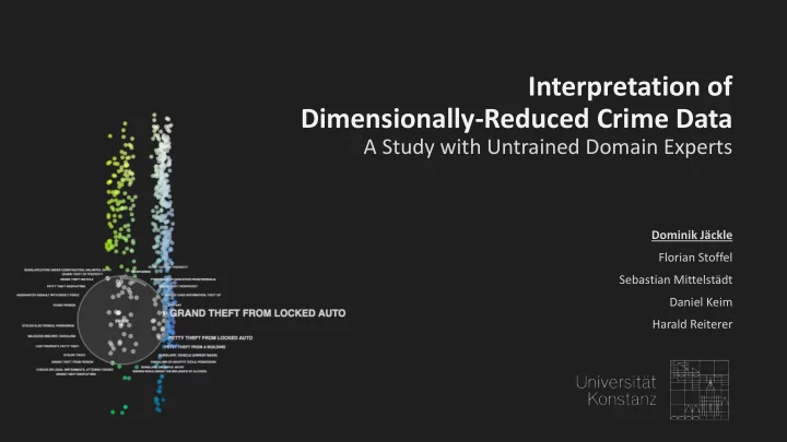
Interpretation of Dimensionally-Reduced Crime Data
A Study with Untrained Domain Experts
Dominik Jäckle Florian Stoffel Sebastian Mittelstädt Daniel Keim Harald Reiterer
Interpretation of Dimensionally-Reduced Crime Data A Study with - - PowerPoint PPT Presentation
Interpretation of Dimensionally-Reduced Crime Data A Study with Untrained Domain Experts Dominik Jckle Florian Stoffel Sebastian Mittelstdt Daniel Keim Harald Reiterer Introduction to Domain Experts Data analysts of a Law Enforcement
Dominik Jäckle Florian Stoffel Sebastian Mittelstädt Daniel Keim Harald Reiterer
Jäckle et al. | Interpretation of Dimensionally-Reduced Crime Data
Jäckle et al. | Interpretation of Dimensionally-Reduced Crime Data
Jäckle et al. | Interpretation of Dimensionally-Reduced Crime Data
Multidimensional Scaling (MDS) = Distance-Preserving Projection A ... ... ... B ... ... ... C ... ... ...
Data Records = Crimes n Attributes
Data
Overall goal: ℝ𝑜 → ℝ𝑛 ; 𝑛 < 𝑜
Jäckle et al. | Interpretation of Dimensionally-Reduced Crime Data
Multidimensional Scaling (MDS) = Distance-Preserving Projection A ... ... ... B ... ... ... C ... ... ...
Data Records = Crimes n Attributes
A B C A 0 ... ... B ... 0 ... C ... ... 0 Data Distance Matrix
Overall goal: ℝ𝑜 → ℝ𝑛 ; 𝑛 < 𝑜
Compute Distances
Jäckle et al. | Interpretation of Dimensionally-Reduced Crime Data
A B C
Multidimensional Scaling (MDS) = Distance-Preserving Projection A ... ... ... B ... ... ... C ... ... ...
Data Records = Crimes n Attributes
A B C A 0 ... ... B ... 0 ... C ... ... 0 Data Distance Matrix 2D Scatterplot
Overall goal: ℝ𝑜 → ℝ𝑛 ; 𝑛 < 𝑜
Compute Distances Projection
Jäckle et al. | Interpretation of Dimensionally-Reduced Crime Data
Jäckle et al. | Interpretation of Dimensionally-Reduced Crime Data
Ward & Martin (1995) Buja (1996)
Jäckle et al. | Interpretation of Dimensionally-Reduced Crime Data
Ward & Martin (1995) Buja (1996)
Seo & Shneiderman (2005) Nam & Mueller (2013) Krause et al. (2016)
Application Examples Case Studies
Johansson & Johansson (2009) Ingram et al. (2010) Turkay et al. (2011) Fernstad et al. (2013) Turkay et al. (2012) Yuan et al. (2013) Liu et al. (2014) Jeong et al. (2009)
User Studies
without Domain Experts
Yi et al. (2005) Brown et al. (2012) Sedlmair et al. (2013) Stahnke et al. (2016)
https://data.sfgov.org/ Category Description DayOfWeek Date Time PdDistrict Resolution Address Location
Category Description DayOfWeek Date Time PdDistrict Resolution Address Location
Category: DISORDERLY CONDUCT Description: MAINTAINING A PUBLIC NUISANCE AFTER NOTIFICATION DayOfWeek: Sunday Date: 08/21/2016 12:00:00 AM Time: 6:36 PdDistrict: TENDERLOIN Resolution: ARREST, BOOKED Address: 400 Block of LEAVENWORTH ST Location: (37.7851373814889°, -122.414457162309°)
https://data.sfgov.org/
Jäckle et al. | Interpretation of Dimensionally-Reduced Crime Data
DISORDERLY CONDUCT MAINTAINING A PUBLIC NUISANCE AFTER NOTIFICATION 08/21/2016 00:06:36 AM categorical numerical textual
Jäckle et al. | Interpretation of Dimensionally-Reduced Crime Data
DISORDERLY CONDUCT MAINTAINING A PUBLIC NUISANCE AFTER NOTIFICATION 08/21/2016 00:06:36 AM categorical numerical textual
1, 𝑊 2 = 𝑊 1 − 𝑊 2
𝑤1∙𝑤2 𝑤1 ∙ 𝑤2
1, 𝑊 2 = 𝑊 1 ≠ 𝑊 2
Dimension/Variable
𝐸1 𝑡𝑗𝑛1 𝑥1 𝐸2 𝑡𝑗𝑛2 𝑥2 𝐸3 𝑡𝑗𝑛3 𝑥3 … 𝐸𝑜 𝑡𝑗𝑛𝑜 𝑥𝑜
Weighting & Similarity Visual Data Exploration
Projection Steering
Jäckle et al. | Interpretation of Dimensionally-Reduced Crime Data
σ𝑗=1
|𝑒𝑗𝑛| 𝑡𝑗𝑛𝑗 𝐵𝑗,𝐶𝑗 ∙𝑥𝑗
|𝑒𝑗𝑛|
Jäckle et al. | Interpretation of Dimensionally-Reduced Crime Data
𝑒𝑗𝑡𝑢 𝐵, 𝐶 = σ𝑗=1
|𝑒𝑗𝑛| 𝑡𝑗𝑛𝑗 𝐵𝑗, 𝐶𝑗 ∙ 𝑥𝑗
|𝑒𝑗𝑛|
Jäckle et al. | Interpretation of Dimensionally-Reduced Crime Data
Jäckle et al. | Interpretation of Dimensionally-Reduced Crime Data
Jäckle et al. | Interpretation of Dimensionally-Reduced Crime Data
Jäckle et al. | Interpretation of Dimensionally-Reduced Crime Data
𝑒𝑗𝑡𝑢 𝐵, 𝐶 = σ𝑗=1
|𝑒𝑗𝑛| 𝑡𝑗𝑛𝑗 𝐵𝑗, 𝐶𝑗 ∙ 𝑥𝑗
|𝑒𝑗𝑛|
Jäckle et al. | Interpretation of Dimensionally-Reduced Crime Data
3 LEA data analysts (1 female)
4 consecutive tasks
Jäckle et al. | Interpretation of Dimensionally-Reduced Crime Data
San Francisco Crime Data
After the study, we let analysts fill out a questionaire regarding:
Jäckle et al. | Interpretation of Dimensionally-Reduced Crime Data
Jäckle et al. | Interpretation of Dimensionally-Reduced Crime Data
Jäckle et al. | Interpretation of Dimensionally-Reduced Crime Data
Jäckle et al. | Interpretation of Dimensionally-Reduced Crime Data
Jäckle et al. | Interpretation of Dimensionally-Reduced Crime Data
Jäckle et al. | Interpretation of Dimensionally-Reduced Crime Data
Dominik Jäckle Florian Stoffel Sebastian Mittelstädt Daniel Keim Harald Reiterer
http://www.dominikjaeckle.com/projects/2017/crime_interpret