International Trade: Theory and Evidence Growth in world exports: - - PowerPoint PPT Presentation

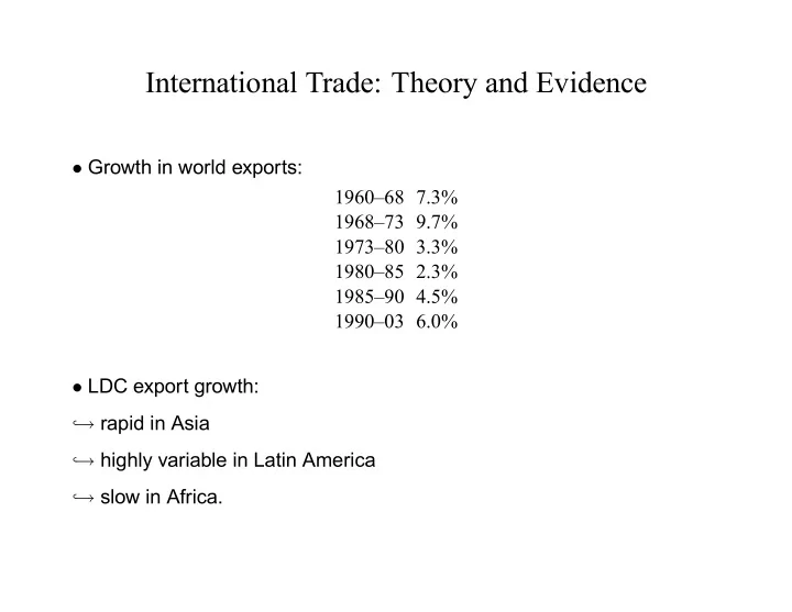
International Trade: Theory and Evidence

• Growth in world exports:

1960–68 7.3% 1968–73 9.7% 1973–80 3.3% 1980–85 2.3% 1985–90 4.5% 1990–03 6.0%

• LDC export growth:

, → rapid in Asia , → highly variable in Latin America , → slow in Africa.

• 10 -

Figure 1. Growth of Merchandise Exports, 1970-20001

100 600 1100 1600 2100 2600 1970 1975 1980 1985 1990 1995 2000 index (1980=100) World

Source: IMF World Economic Outlook (WEO).

1 Excluding oil exports.

Least Developed Countries Other Developing Countries Sub-Saharan Africa

Figure 3. World: Product Composition of Merchandise Exports, 1965-98

10 20 30 40 50 60 70 80 90 100 1965 1970 1975 1980 1985 1990 1995 1998 percent

Agriculture Manufactures Minerals

Source: GTAP database, version 5.

Figure 2. Developing Countries: Share of Exports Going to Other Developing Countries, 1965-98

5 10 15 20 25 30 35 40 45 1965 1970 1975 1980 1985 1990 1995 1998 percent

Minerals Agriculture Manufactures Total Source: Global Trade Analysis Project (GTAP) database, version 5.

• Developing countries’ share of world trade:

, → 20% in 1980 , → 30% in 2005. , → BUT decline in share of sub–saharan Africa (1% → 0.5%)

• Composition of LDC exports has shifted towards manufacturing

, → now about 70% of total exports , → mostly due to East Asia (esp. China) , → often a result of deliberate policies

Figure 4. Developing Countries: Composition of Merchandise Exports, 1965-98

10 20 30 40 50 60 70 80 90 100

1965 1970 1975 1980 1985 1990 1995 1998

percent

Manufactures Agriculture Minerals

Source: GTAP database, version 5.

Figure 5. Share of Commerical Services in Total Exports of Goods and Services,

Figure 6. Sub-Saharan Africa: Composition of Merchandise Exports, 1965-95

10 20 30 40 50 60 70 80 90 100 1965 1970 1975 1980 1985 1990 1995 percent

Manufactures Agriculture Minerals

Source: GTAP database, version 5.

• Standard hypothesis of trade patterns:

DCs Primary goods

¿

Manufactures LDCs

, → LDCs export proportionately more primary goods , → BUT developed countries do not import proportionately more primary

goods Why ?

, → large fraction of DC trade is within DCs and is in manufactured goods

• Actual World trade ßows

DCs

Manufactures

¿

DCs

Primary ↑↓ Manu. Primary ↑↓ Manu.

LDCs

∼

LDCs

• However, trade between LDCs has increased recently to about 10% of

world trade

Why Do Countries Trade ?

• 1. Comparative Advantage — Ricardian Trade Theory

Example:

, → 2 countries: North and South , → 2 goods: Computers and Rice , → 1 factor: labour – 600 workers each

Technological assumptions: Labour One One sack Required Computer

• f Rice

in North 10 15 in South 40 20

, → North has an absolute advantage in both goods, , → but a comparative advantage in computers. , → South has a comparative advantage in rice.

Production possibilities frontier

• In North:

10CN + 15RN = 600 , → can be written as RN = 40 − 2 3CN

• In South

40CS + 20RS = 600 , → can be written as RS = 30 − 2CS

Rice Rice Computers Computers 40 60 30 15

North South

2/3 2

1.Production Possibilities

Autarky

• If both goods are consumed in North:

pN

c

pN

r

= 10 15 = 2 3.

Why?

, → Competition ⇒ pN

c = 10wc

and pN

r = 15wr

If pN

c

10>pN

r

15, then wc > wr

, → all workers flow into computers.

If pN

c

10 < pN

r

15, then wc < wr

, → all workers flow into rice

For both goods to be produced, we need

wc = wr

• Similarly, if both goods are consumed in South:

pS

c

pS

r

= 40 20 = 2.

Free Trade

• If both goods are going to be produced:

2 3 < pc pr < 2.

Why ? if pc

pr < 2 3 < 2, both countries specialize in rice

if pc

pr > 2 > 2 3, both countries specialize in computers

if 2

3 < pc pr < 2,

, → North specializes in computers , → South specializes in rice.

• If it is cheaper to produce rice in North, why don’t people buy rice there?

, → market wages adjust so that rice is not cheaper in the North. , → as we move from autarky to free trade pN

c ↑

pN

r ↓

pS

c ↓

pS

r ↑

so that North : pN

c

10 = wN > pN

r

15 ⇒ specialize in C

South : pS

c

40 < wS = pS

r

20 ⇒ specialize in C , → effectively nullifies S’s advantage in rice production.

Predictions of Ricardian Theory

• Each country specializes in the production of the goods in which it has a

comparative advantage and exports them in return for other goods.

• All households in both countries are unambiguously better off with free

trade than in autarky.

, → the wage in both countries rises , → consumption possibilities lie outside the production possibilities frontier

Caveats

• only one factor of production
• labour is perfectly mobile across sectors
• competitive markets

Rice Rice Computers Computers

North South

Consumption Consumption Production pc/pr pc/pr X M X M

2.Gains From Trade

• 2. Factor Endowments — Neoclassical Trade Theory

(Eli Heckscher and Bertil Ohlin) Example

, → 2 countries: North and South , → 2 goods: Cars and Textiles , → 2 factors: Capital (K) and Labour (L) , → identical preferences across countries

• North is relatively well endowed with K :

KN LN > KS LS

• Car production is capital intensive and textile production is labour

intensive.

, → given the same w/r. production isoquants are such that K/L for cars

exceeds textiles

w/r Capital Labour Kc / Lc KT / LT Cars Textiles isocost line

3.Capital Intensity

A B C 0C 0T Capital Labour

4.Edgeworth box for North

Textiles Cars A B C

5.Production Possibilities Frontier for North

Capital Labour 0C 0T D E F

6.Edgeworth Box for South

Textiles Cars D E F

7.PPF for South

Textiles Cars C pC/pT

N N

P Excess Supply Excess Demand

8.Disequilibrium in Autarky

Textiles Cars pC/pT

N N

E T* C*

9.Equilibrium under Autarky

pC/pT pC/pT

N N S S

10.Autarky in North and South

pC/pT pC/pT

North South

CN PN CS PN X M X M

11.Free Trade Equilibrium

Implications of Neoclassical Trade Theory

• Under free trade the price ratio settles at a level between the two autarkic

price ratios

• Incomplete specialization — both countries produce both goods
• A country will tend to export the commodities that are intensive in factors

that are possessed by that country in relative abundance.

, → consistent with the “standard hypothsis” of DC–LDC trade, , → does not explain trade flows amongst OECD countries , → model predicts a lot of trade between DCs and LDCs

• Households in both countries are potentially better off with free trade

BUT there are distributional consequences

• 3. Differences in Preferences
• How do preferences differ between LDCs and DCs ?

, → one hypothesis: DCs spend proportionately more on manufactured

goods (luxuries)

, → drives down relative price of primary goods as DCs get richer

pC/pT pC/pT Textiles Textiles Cars Cars M M X X

12.Trade due to differences in preferences

• 4. Economies of Scale
• Trade allows concentration of production in some coutries to maximize

the effects of economies of scale Example:

, → 2 identical countries — East and West , → 2 goods — ships and aircraft

Aircraft Ships AC AC $ $ A B C D Autarky

13.Trade and Specialization with Economies of Scale

The Gains and Losses from Trade Distributional Consequences of Trade

• Neoclassical theory ⇒ potential gains due to increased goods/services

BUT not necessarily actual gains to all members of society. Example (from earlier): Move toward free trade in North

, → increased (capital–intensive) car production , → reduced (labour–intensive) textile production ⇒ w/r falls , → i.e. labour loses, capital gains

• Distribution of gains depends on distribution of factor ownership

Static vs. Dynamic Gains/Losses from Trade

• Comparative advantage is a static concept

, → but technologies and factor endowments change over time

• LDCs could allow trade patterns to change as they accumulate physical

/ human capital

, → “natural” shift from primary to manufacturing

BUT may get stuck as primary producer and never invest enough to get beyond this stage

Why ? — Prebisch–Singer Hypothesis

, → as world gets richer, fraction of income spent on primary products

declines

, → long–term deterioration in the terms of trade faced by many LDCs:

T.o.T. = Export Price Index Import Price Index

⇒ real incomes grow less rapidly , → less capital accumulation / infrastructure

• Policy implication: need to protect / promote domestic manufacturing

, → may lower current income by distorting the gains from trade , → but this is an “investment” which will raise future incomes.

Does this hypothesis make any sense?

• not necessary that world demand will go against primary products (e.g.

coffee beans)

, → BUT slow recovery from 60% decline in early 1980s,

• policy implication assumes that capital markets are not working properly

, → in a functioning capital market, high future returns in manfacturing

should induce investment flow into it and away from primary production.

Figure 1. Evolution of non-oil commodity terms of trade

Indices 1980 = 100; prices deflated by the unit value of manufactures exports from the G-5 countries to developing countries

Table 1 World Bank commodity price indices for low and middle income countries (1990 =100)

1970 1980 1990 2000 Jan-Dec 2002 Jan-Dec 2003 Jan-May 2004 Agriculture 163.3 175.2 100.0 93.0 86.4 94.7 107.1 Beverages 202.8 230.2 100.0 90.9 84.6 87.1 90.3 Food 166.5 176.7 100.0 87.0 90.1 96.4 116.0 Fats and Oils 229.5 188.6 100.0 99.0 101.2 120.6 157.5 Grains 166.6 170.4 100.0 81.8 88.1 90.2 104.2 Other Food 114.9 170.5 100.0 80.0 82.1 80.1 88.7 Source: 1970-2000: World Bank Global Economic Prospects 2004 (Appendix 2) 2002-2004: World Bank Commodity Price Data Pinksheet - June 2004 40 60 80 100 1980 1982 1984 1986 1988 1990 1992 1994 1996 1998 2000

Sub-Saharan Afric a Developin g countri es

Figure 1.21 Commodity prices continued gains through 2007 led by metals

Source: World Bank.

J a n . 1 , 2 J a n . 1 , 2 1 J a n . 1 , 2 2 J a n . 1 , 2 3 J a n . 1 , 2 4 J a n . 1 , 2 5 J a n . 1 , 2 6 J a n . 1 , 2 7

350 50 300 250 200 150 100 Metals Crude oil Agriculture Commodity price indexes (January 2003 100)

Figure 1.22 Copper, zinc, and aluminum prices sharply affected by China

Sources: London Mercantile Exchange and World Bank. J a n . 3 , 2 J a n . 3 , 2 1 J a n . 3 , 2 2 J a n . 3 , 2 3 J a n . 3 , 2 4 J a n . 3 , 2 5 J a n . 3 , 2 6 J a n . 3 , 2 7 9,000 7,000 8,000 5,000 6,000 3,000 4,000 2,000 1,000 Copper Aluminum Zinc $/metric ton

growing conditions in India, Pakistan, and Thailand improved, and new plantings and fa- vorable weather boosted Brazilian production. Food prices have risen nearly 75 percent since their lows of 2000. The increases stem partly from the stepped-up use of food crops for biofuels and partly from other more fundamen- tal factors, such as rapid income growth in de- veloping countries, high fertilizer prices, low stocks, and droughts. Biofuels are playing an increasingly important role in agricultural commodity markets as their share of global production and trade increases. In 2006, bio- fuels accounted for 5–10 percent of the global production of the primary biofuel feedstocks and up to 77 percent of the volume of trade. Among the largest biofuel producers, the United States used 20 percent of its maize pro- duction for biofuels; Brazil used 50 percent of its sugarcane for biofuels; and the EU used 68 percent of its vegetable oil production, primarily rapeseed, and also imported addi- tional vegetable oils. Such large usage reduces supplies of these crops for food and feed and has contributed to substantial price gains (box 1.2). The anticipated spike in grains prices, iden- tified as a concern in the World Bank’s Global Development Finance report published in May 2007 (World Bank 2007a), has largely

• materialized. Monthly wheat prices have in-

creased 90 percent since mid-2007. Wheat stocks are expected to fall to record lows rela- tive to consumption, and prices may increase further in 2008 before production recoups enough to rebuild stocks. In the meantime, a large number of food-importing countries may suffer substantial terms-of-trade losses

• ver the course of 2007 and into 2008 (box

1.3). Price increases for vegetable oils and grains primarily affect low-income countries, with the rise in prices since the end of 2004 leading to a terms-of-trade loss equivalent to 0.5 percent of GDP. This represents 1 percent

• f GDP in 29 countries, and nearly 5 percent
• f GDP for the most affected country, Eritrea.

The impact on middle- and high-income coun- tries is considerably less because imports of these commodities represent a smaller share of trade, and higher prices on other commodity exports tends to offset terms-of-trade losses resulting from higher food prices. Agricultural prices are expected to remain nearly flat at high levels in 2008, as biofuels production continues to ramp up in response to consump- tion mandates and production subsidies, drawing resources from other crops.

Figure 1.26 A rise in food price led by a ramp-up of the prices of fats, oils, and grains

Source: World Bank.

J a n . 1 , 2 J a n . 1 , 2 1 J a n . 1 , 2 2 J a n . 1 , 2 3 J a n . 1 , 2 4 J a n . 1 , 2 5 J a n . 1 , 2 6 J a n . 1 , 2 7

200 50 175 125 150 75 100 Fats and oils Other foods Commodity price indexes (1990 100) Grains

Figure 1.25 Agricultural prices surge over 2006–7

Source: World Bank.

J a n . 1 , 2 J a n . 1 , 2 1 J a n . 1 , 2 2 J a n . 1 , 2 3 J a n . 1 , 2 4 J a n . 1 , 2 5 J a n . 1 , 2 6 J a n . 1 , 2 7

175 50 150 100 125 75 Raw materials Food Beverages Commodity price indexes (2003 100)

BUT there are many market failures

, → imperfect capital markets create bias against future benefits relative

to current costs.

, → dynamic gains from investment may involve positive externalities , → distribution of wealth , → large country tariff argument ⇒ may justify government intervention in the form of trade policy.