Important Terms in Probability I Random Experiment it is a process - - PowerPoint PPT Presentation

Statistics for Business

Elements of Probability Theory Panagiotis Th. Konstantinou

MSc in International Shipping, Finance and Management, Athens University of Economics and Business

First Draft: July 15, 2015. This Draft: September 3, 2020.

• P. Konstantinou (AUEB)

Statistics for Business – I September 3, 2020 1 / 38 Elements of Probability Theory Sets

Important Terms in Probability – I

Random Experiment – it is a process leading to an uncertain

• utcome

Basic Outcome (Si) – a possible outcome (the most basic one) of a random experiment Sample Space (S) – the collection of all possible (basic) outcomes

• f a random experiment

Event A – is any subset of basic outcomes from the sample space (A ⊆ S). This is our object of interest here – among other things.

• P. Konstantinou (AUEB)

Statistics for Business – I September 3, 2020 2 / 38 Elements of Probability Theory Sets

Important Terms in Probability – II



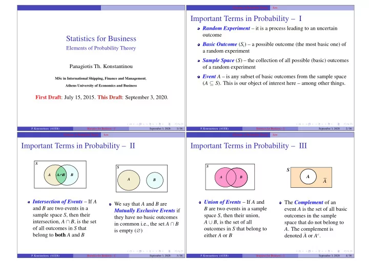
∩ A B A∩B S

Intersection of Events – If A and B are two events in a sample space S, then their intersection, A ∩ B, is the set

• f all outcomes in S that

belong to both A and B





∩

A B S

We say that A and B are Mutually Exclusive Events if they have no basic outcomes in common i.e., the set A ∩ B is empty (∅)

• P. Konstantinou (AUEB)

Statistics for Business – I September 3, 2020 3 / 38 Elements of Probability Theory Sets

Important Terms in Probability – III



∪ A B S

Union of Events – If A and B are two events in a sample space S, then their union, A ∪ B, is the set of all

• utcomes in S that belong to

either A or B



A S

A

The Complement of an event A is the set of all basic

• utcomes in the sample

space that do not belong to

• A. The complement is

denoted ¯ A or Ac.

• P. Konstantinou (AUEB)

Statistics for Business – I September 3, 2020 4 / 38

Elements of Probability Theory Sets

Important Terms in Probability – IV

Events E1, E2, ..., Ek are Collectively Exhaustive events if E1 ∪ E2 ∪ ... ∪ Ek = S, i.e., the events completely cover the sample space.

Examples

Let the Sample Space be the collection of all possible outcomes of rolling one die S = {1, 2, 3, 4, 5, 6}. Let A be the event “Number rolled is even”: A = {2, 4, 6} Let B be the event “Number rolled is at least 4” : B = {4, 5, 6} Mutually exclusive: A and B are not mutually exclusive. The

• utcomes 4 and 6 are common to both.
• P. Konstantinou (AUEB)

Statistics for Business – I September 3, 2020 5 / 38 Elements of Probability Theory Sets

Important Terms in Probability – V

Examples (Continued)

A = {2, 4, 6} B = {4, 5, 6} Collectively exhaustive: A and B are not collectively exhaustive. A ∪ B does not contain 1 or 3. Complements: ¯ A = {1, 3, 5} and ¯ B = {1, 2, 3} Intersections: A ∩ B = {4, 6}; ¯ A ∩ B = {5}; A ∩ ¯ B = {2}; ¯ A ∩ ¯ B = {1, 3}. Unions: A ∪ B = {2, 4, 5, 6}; A ∪ ¯ A = {1, 2, 3, 4, 5, 6} = S.

• P. Konstantinou (AUEB)

Statistics for Business – I September 3, 2020 6 / 38 Elements of Probability Theory Probability

Assessing Probability – I

Probability – the chance that an uncertain event A will occur is always between 0 and 1.

• Impossible

≤ Pr(A) ≤ 1

• Certain

There are three approaches to assessing the probability of an uncertain event:

• P. Konstantinou (AUEB)

Statistics for Business – I September 3, 2020 7 / 38 Elements of Probability Theory Probability

Assessing Probability – II

1

Classical Definition of Probability: Probability of an event A = NA N = number of outcomes that satisfy the event A total number of outcomes in the sample space S

◮ Assumes all outcomes in the sample space are equally likely to

• ccur.

◮ Example: Consider the experiment of tossing 2 coins. The sample space is S = {HH, HT, TH, TT}. ◮ Event A = {one T} = {TH, HT}. Hence Pr(A) = 0.5 – assuming that all basic outcomes are equally likely. ◮ Event B = {at least one T} = {TH, HT, TT}. So Pr(B) = 0.75.

• P. Konstantinou (AUEB)

Statistics for Business – I September 3, 2020 8 / 38

Elements of Probability Theory Probability

Assessing Probability – III

2

Probability as Relative Frequency: Probability of an event A = nA n = number of events in the population that satisfy event A total number of events in the population

◮ The limit of the proportion of times that an event A occurs in a large number of trials, n.

• P. Konstantinou (AUEB)

Statistics for Business – I September 3, 2020 9 / 38 Elements of Probability Theory Probability

Assessing Probability – IV

3

Subjective Probability: an individual has opinion or belief about the probability of occurrence of A.

◮ When economic conditions or a company’s circumstances change rapidly, it might be inappropriate to assign probabilities based solely on historical data ◮ We can use any data available as well as our experience and intuition, but ultimately a probability value should express our degree of belief that the experimental outcome will occur.

• P. Konstantinou (AUEB)

Statistics for Business – I September 3, 2020 10 / 38 Elements of Probability Theory Probability

Measuring Outcomes – I

Classical Definition of Probability

Basic Rule of Counting: If an experiment consists of a sequence

• f k steps in which there are n1 possible results for the first step,

n2 possible results for the second step, and so on, then the total number of experimental outcomes is given by (n1)(n2)...(nk) – tree diagram...

• P. Konstantinou (AUEB)

Statistics for Business – I September 3, 2020 11 / 38 Elements of Probability Theory Probability

Measuring Outcomes – II

Classical Definition of Probability

Counting Rule for Combinations (Number of Combinations of n Objects taken k at a time): A second useful counting rule enables us to count the number of experimental outcomes when k objects are to be selected from a set of n objects (the ordering does not matter) Cn

k =

n k

• =

n! k!(n − k)!, where n! = n(n − 1)(n − 2)...(2)(1) and 0! = 1.

• P. Konstantinou (AUEB)

Statistics for Business – I September 3, 2020 12 / 38

Elements of Probability Theory Probability

Measuring Outcomes – III

Classical Definition of Probability

◮ Example: Suppose we flip three coins. How many are the possible combinations with (exactly) 1 T? C3

1 =

3 1

• =

3! 1!(3 − 1)! = 3. ◮ Example: Suppose we flip three coins. How many are the possible combinations with at least 1T? ◮ Example: Suppose that there are two groups of questions. Group A with 6 questions and group B with 4 questions. How many are the possible half-a-dozens we can put together? n = 6 + 4 = 10; C10

6 =

10 6

• =

10! 6!(10 − 6)! = 210.

• P. Konstantinou (AUEB)

Statistics for Business – I September 3, 2020 13 / 38 Elements of Probability Theory Probability

Measuring Outcomes – IV

Classical Definition of Probability

◮ Example: How many possible half-a-dozens we can put together, preserving the ratio 4 : 2? 6 4

• ×

4 2

• = 15 × 6 = 90.

◮ Probability: What is the probability of selecting a particular half-a-dozen (with ratio 4 : 2), when we choose at random? Using the classical definition of probability 90 210 = 0.4286

• P. Konstantinou (AUEB)

Statistics for Business – I September 3, 2020 14 / 38 Elements of Probability Theory Probability

Measuring Outcomes – V

Classical Definition of Probability

Counting Rule for Permutations (Number of Permutations of n Objects taken k at a time): A third useful counting rule enables us to count the number of experimental outcomes when k objects are to be selected from a set of n objects, where the order of selection is important Pn

k =

n! (n − k)!.

• P. Konstantinou (AUEB)

Statistics for Business – I September 3, 2020 15 / 38 Elements of Probability Theory Probability

Measuring Outcomes – VI

Classical Definition of Probability

◮ Example: How many 3-digit lock combinations can we make from the numbers 1, 2, 3, and 4? The order of the choice is important! So P4

3 = 4!

1! = 4! = 4(3)(2)(1) = 24. ◮ Example: Let the characters A, B, Γ. In how many ways can we combine them in making triads? P3

3 = 3!

0! = 3! = 3(2)(1) = 6. These are: ABΓ, AΓB, BAΓ, BΓA, ΓAB,and ΓBA.

• P. Konstantinou (AUEB)

Statistics for Business – I September 3, 2020 16 / 38

Elements of Probability Theory Probability

Measuring Outcomes – VII

Classical Definition of Probability

◮ Example: Let the characters A, B, Γ, ∆, E. In how many ways is it possible to combine them into pairs? ∗ If the order matters, we may have P5

2 = 5!

3! = (5)(4) = 20. ∗ If the order does not matters, we may choose pairs C5

2 =

5 2

• =

5! 2!(5 − 2)! = 5! 2!3! = 10

• P. Konstantinou (AUEB)

Statistics for Business – I September 3, 2020 17 / 38 Elements of Probability Theory Axioms and Rules of Probability

Probability Axioms

The following Axioms hold

1

If A is any event in the sample space S, then 0 ≤ Pr(A) ≤ 1.

2

Let A be an event in S, and let Si denote the basic outcomes. Then Pr(A) =

• all Si in A

Pr(Si).

3

Pr(S) = 1.

• P. Konstantinou (AUEB)

Statistics for Business – I September 3, 2020 18 / 38 Elements of Probability Theory Axioms and Rules of Probability

Probability Rules – I

The Complement Rule: Pr(¯ A) = 1 − Pr(A) [i.e., Pr(A) + Pr(¯ A) = 1]. The Addition Rule: The probability of the union of two events is Pr(A ∪ B) = Pr(A) + Pr(B) − Pr(A ∩ B) Probabilities and joint probabilities for two events A and B are summarized in the following table: B ¯ B A Pr(A ∩ B) Pr(A ∩ ¯ B) Pr(A) ¯ A Pr(¯ A ∩ B) Pr(¯ A ∩ ¯ B) Pr(¯ A) Pr(B) Pr(¯ B) Pr(S) = 1

• P. Konstantinou (AUEB)

Statistics for Business – I September 3, 2020 19 / 38 Elements of Probability Theory Axioms and Rules of Probability

Probability Rules – II

Example (Addition Rule)

Consider a standard deck of 52 cards, with four suits ♥♣♦♠. Let event A = card is an Ace and event B = card is from a red suit.

Pr(Red ∪ Ace) = Pr(Red) + Pr(Ace) - Pr(Red ∩ Ace) = 26/52 + 4/52 - 2/52 = 28/52

Don’t count the two red aces twice!

Black

Color Type

Red

Total Ace 2 2 4 Non-Ace 24 24 48 Total 26 26 52

• P. Konstantinou (AUEB)

Statistics for Business – I September 3, 2020 20 / 38

Elements of Probability Theory Axioms and Rules of Probability

Conditional Probability – I

A conditional probability is the probability of one event, given that another event has occurred: Pr(A|B) = Pr(A ∩ B) Pr(B) (if Pr(B) > 0); Pr(B|A) = Pr(A ∩ B) Pr(A) (if Pr(A) > 0)

• P. Konstantinou (AUEB)

Statistics for Business – I September 3, 2020 21 / 38 Elements of Probability Theory Axioms and Rules of Probability

Conditional Probability – II

Example (Conditional Probability)

Of the cars on a used car lot, 70% have air conditioning (AC) and 40% have a CD player (CD). 20% of the cars have both. What is the probability that a car has a CD player, given that it has AC? [Pr(CD|AC) =?]

No CD CD Total

AC .2 .5 .7 No AC .2 .1 .3 Total .4 .6 1.0



Pr(CD AC) .2 Pr(CD|AC) .2857 Pr(AC) .7 ∩ = = =

• P. Konstantinou (AUEB)

Statistics for Business – I September 3, 2020 22 / 38 Elements of Probability Theory Axioms and Rules of Probability

Multiplication Rule

The Multiplication Rule for two events A and B: Pr(A ∩ B) = Pr(A|B) Pr(B) = Pr(B|A) Pr(A)

Example (Multiplication Rule)

Pr(Red ∩ Ace) = Pr(Red| Ace)Pr(Ace) Black

Color Type

Red

Total Ace 2 2 4 Non-Ace 24 24 48 Total 26 26 52

52 2 52 4 4 2 =             =

52 2 cards

• f

number total ace and red are that cards

• f

number = =

• P. Konstantinou (AUEB)

Statistics for Business – I September 3, 2020 23 / 38 Elements of Probability Theory Independence, Joint and Marginal Probabilities

Statistical Independence – I

Two events are statistically independent if and only if: Pr(A ∩ B) = Pr(A) Pr(B).

◮ Events A and B are independent when the probability of one event is not affected by the other event. ◮ If A and B are independent, then Pr(A|B) = Pr(A), if Pr(B) > 0; Pr(B|A) = Pr(B), if Pr(A) > 0.

• P. Konstantinou (AUEB)

Statistics for Business – I September 3, 2020 24 / 38

Elements of Probability Theory Independence, Joint and Marginal Probabilities

Statistical Independence – II

Example (Statistical Independence)

Of the cars on a used car lot, 70% have air conditioning (AC) and 40% have a CD player (CD). 20% of the cars have both. Are the events AC and CD statistically independent?

No CD CD Total

AC .2 .5 .7 No AC .2 .1 .3 Total .4 .6 1.0

P(AC ∩ CD) = 0.2 P(AC) = 0.7 P(CD) = 0.4 P(AC)P(CD) = (0.7)(0.4) = 0.28 P(AC ∩ CD) = 0.2 ≠ P(AC)P(CD) = 0.28 So the two events are not statistically independent

• P. Konstantinou (AUEB)

Statistics for Business – I September 3, 2020 25 / 38 Elements of Probability Theory Independence, Joint and Marginal Probabilities

Statistical Independence – III

Remark (Exclussive Events and Statistical Independence)

Let two events A and B with Pr(A) > 0 and Pr(B) > 0 which are mutually exclusive. Are A and B independent? NO! To see this use a Venn diagram and the formula of conditional probability (or the multiplication rule). If one mutually exclusive event is known to occur, the other cannot occur; thus, the probability of the other event occurring is reduced to zero (and they are therefore dependent).

• P. Konstantinou (AUEB)

Statistics for Business – I September 3, 2020 26 / 38 Elements of Probability Theory Independence, Joint and Marginal Probabilities

Examples – I

Example 1. In a certain population, 10% of the people can be classified as being high risk for a heart attack. Three people are randomly selected from this population. What is the probability that exactly one of the three are high risk? ◮ Define H: high risk, and N: not high risk. Then Pr(exactly one high risk) = Pr(HNN) + Pr(NHN) + Pr(NNH) = = Pr(H) Pr(N) Pr(N) + Pr(N) Pr(H) Pr(N) + Pr(N) Pr(N) Pr(H) = (.1)(.9)(.9) + (.9)(.1)(.9) + (.9)(.9)(.1) = 3(.1)(.9)2 = .243

• P. Konstantinou (AUEB)

Statistics for Business – I September 3, 2020 27 / 38 Elements of Probability Theory Independence, Joint and Marginal Probabilities

Examples – II

Example 2. Suppose we have additional information in the previous example. We know that only 49% of the population are

• female. Also, of the female patients, 8% are high risk. A single

person is selected at random. What is the probability that it is a high risk female? ◮ Define H: high risk, and F: female. From the example, Pr(F) = .49 and Pr(H|F) = .08. Using the Multiplication Rule: Pr(high risk female) = Pr(H ∩ F) = Pr(F) Pr(H|F) = .49(.08) = .0392

• P. Konstantinou (AUEB)

Statistics for Business – I September 3, 2020 28 / 38

Elements of Probability Theory Independence, Joint and Marginal Probabilities

Joint and Marginal Probabilities – I

The Law of Total Probability

Recall that the probability of a joint event, A ∩ B is Pr(A ∩ B) = number of outcomes satisfying A and B total number of elementary outcomes . Let S1, S2, S3, ..., Sk be mutually exclusive and exhaustive events (that is, one and only one must happen). Then the probability of another event A (marginal probability) can be written as Pr(A) = Pr(A ∩ S1) + Pr(A ∩ S2) + ... + Pr(A ∩ Sk)

• P. Konstantinou (AUEB)

Statistics for Business – I September 3, 2020 29 / 38 Elements of Probability Theory Independence, Joint and Marginal Probabilities

Joint and Marginal Probabilities – II

The Law of Total Probability

Από κοινού ( πιθανότητες και περιθωρίου πιθανότητες

1 2 3

Pr( ) Pr( ) Pr( ) Pr( ) A A S A S A S = ∩ + ∩ + ∩

S1 S2 S3 Α∩S1 Α∩S2 Α∩S3

Α=ελαττωματικό, Β=παραγωγή μηχανής

• P. Konstantinou (AUEB)

Statistics for Business – I September 3, 2020 30 / 38 Elements of Probability Theory Independence, Joint and Marginal Probabilities

Joint and Marginal Probabilities – III

The Law of Total Probability

Example (Total Probability)

P(Ace) Black

Color Type

Red

Total Ace 2 2 4 Non-Ace 24 24 48 Total 26 26 52

2 2 4 Pr(Ace Red) Pr(Ace Black) 52 52 52 = ∩ + ∩ = + =

• P. Konstantinou (AUEB)

Statistics for Business – I September 3, 2020 31 / 38 Elements of Probability Theory Bayes Rule

Bayes Rule – I

Bayes’ Theorem: Let S1, S2, S3, ..., Sk be mutually exclusive and exhaustive events with prior probabilities Pr(S1), Pr(S2), . . . , Pr(Sk). If an event A occurs, the posterior probability of Si, given that A occurred is Pr(Si|A) = Pr(Si) Pr(A|Si) k

i=1 Pr(Si) Pr(A|Si)

for i = 1, 2, ..., k. Idea:

◮ We begin a probability analysis with initial or prior probabilities. ◮ Then, from a sample, special report, or a product test we obtain some additional information. ◮ Given this information, we calculate revised or posterior probabilities.

• P. Konstantinou (AUEB)

Statistics for Business – I September 3, 2020 32 / 38

Elements of Probability Theory Bayes Rule

Bayes Rule – II

Example

From a previous example, we know that 49% of the population are

• female. Of the female patients, 8% are high risk for heart attack, while

12% of the male patients are high risk. A single person is selected at random and found to be high risk. What is the probability that it is a male? Define H: high risk; F: female; and M: male We know Pr(F) = .49; Pr(M) = .51; Pr(H|F) = .08; Pr(H|M) = .12. So Pr(M|H) = Pr(M) Pr(H|M) Pr(M) Pr(H|M) + Pr(F) Pr(H|F) = (.51)(.12) (.51)(.12) + (.49)(.08) = 0.61

• P. Konstantinou (AUEB)

Statistics for Business – I September 3, 2020 33 / 38 Elements of Probability Theory Bayes Rule

Bayes Rule: Step-by-Step Example – I

A proposed shopping center will provide strong competition for downtown businesses like L. S. Clothiers. If the shopping center is built, the owner of L. S. Clothiers feels it would be best to relocate to the shopping center. The shopping center cannot be built unless a zoning change is approved by the town council. The planning board must first make a recommendation, for or against the zoning change, to the council.

• P. Konstantinou (AUEB)

Statistics for Business – I September 3, 2020 34 / 38 Elements of Probability Theory Bayes Rule

Bayes Rule: Step-by-Step Example – II

Forming Priors: Let A1 = town council approves the zoning change A2 = town council disapproves the zoning change with (subjective judgement) prior beliefs Pr(A1) = 0.7 and Pr(A2) = 0.3 New Information: The planning board has recommended against the zoning change. Let B denote the event of a negative recommendation by the planning board. Given that B has occurred, should L. S. Clothiers revise the probabilities that the town council will approve or disapprove the zoning change?

• P. Konstantinou (AUEB)

Statistics for Business – I September 3, 2020 35 / 38 Elements of Probability Theory Bayes Rule

Bayes Rule: Step-by-Step Example – III

Conditional Probabilities: Past history with the planning board and the town council indicates the following Pr(B|A1) = Pr(Negative Recom.|Approval of Change) = 0.2, Pr(B|A2) = Pr(Negative Recom.|Disapproval of Change) = 0.9; hence: Pr(¯ B|A1) = Pr(Positive Recom.|Approval of Change) = 0.8, Pr(¯ B|A2) = Pr(Positive Recom.|Disapproval of Change) = 0.1.

• P. Konstantinou (AUEB)

Statistics for Business – I September 3, 2020 36 / 38

Elements of Probability Theory Bayes Rule

Bayes Rule: Step-by-Step Example – IV

P( |A1) = .8 P(A1) = .7 P(A2) = .3 P(B|A2) = .9 P( |A2) = .1 P(B|A1) = .2 P(A1 ∩ B) = .14 P(A2 ∩ B) = .27 P(A2 ∩ ) = .03 P(A1 ∩ ) = .56 Town Council Planning Board Experimental Outcomes  1.00 B B B B

Bayes’ Theorem: To find the posterior probability that event Ai will occur given that event B has occurred, we apply Bayes’ theorem.

• P. Konstantinou (AUEB)

Statistics for Business – I September 3, 2020 37 / 38 Elements of Probability Theory Bayes Rule

Bayes Rule: Step-by-Step Example – V

Posterior Probabilities: Given the planning board’s recommendation not to approve the zoning change, we revise the prior probabilities as follows: Pr(A1|B) = Pr(A1) Pr(B|A1) Pr(A1) Pr(B|A1) + Pr(A2) Pr(B|A2) = (.7)(.2) (.7)(.2) + (.3)(.9) = 0.3415 The planning board’s recommendation is good news for L. S.

• Clothiers. The posterior probability of the town council approving

the zoning change is 0.34 compared to a prior probability of 0.70.

• P. Konstantinou (AUEB)

Statistics for Business – I September 3, 2020 38 / 38