Illustrating Agnostic Learning We want a classifier to distinguish - PowerPoint PPT Presentation

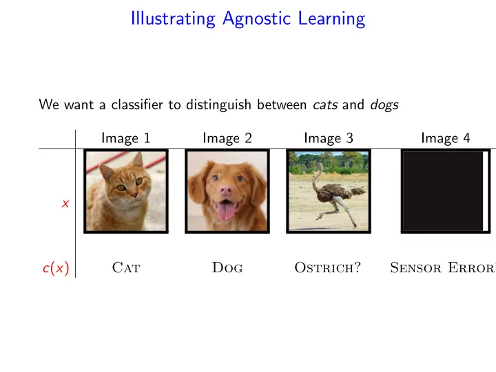
Illustrating Agnostic Learning We want a classifier to distinguish between cats and dogs Image 1 Image 2 Image 3 Image 4 x c ( x ) Cat Dog Ostrich? Sensor Error?

Unrealizable (Agnostic) Learning • We are given a training set { ( x 1 , c ( x 1 )) , . . . , ( x m , c ( x m )) } , and a concept class C • Let c be the correct concept. • Unrealizable case - no hypothesis in the concept class C is consistent with all the training set. • c �∈ C • Noisy labels • Relaxed goal: Find c ′ ∈ C such that D ( c ′ ( x ) � = c ( x )) ≤ inf Pr h ∈C Pr D ( h ( x ) � = c ( x )) + ǫ. • We estimate Pr D ( h ( x ) � = c ( x )) by m � Pr ( h ( x ) � = c ( x )) = 1 ˜ 1 h ( x i ) � = c ( x i ) m i =1

Unrealizable (Agnostic) Learning • We estimate Pr D ( h ( x ) � = c ( x )) by � m Pr ( h ( x ) � = c ( x )) = 1 ˜ 1 h ( x i ) � = c ( x i ) m i =1 • If for all h we have: � � � � � ≤ ǫ � � � � Pr( h ( x ) � = c ( x )) − Pr x ∼D ( h ( x ) � = c ( x )) 2 , then the ERM (Empirical Risk Minimization) algorithm ˆ ˆ h = arg min Pr( h ( x ) � = c ( x )) h ∈C is ǫ -optimal.

More General Formalization • Let f h be the loss (error) function for hypothesis h (often denoted by ℓ ( h , x )). • Here we use the 0-1 loss function: � 0 if h ( x ) = c ( x ) f h ( x ) = 1 if h ( x ) � = c ( x ) • Alternative that gives higher lose to false negative. � 0 if h ( x ) = c ( x ) f h ( x ) = 1 + c ( x ) if h ( x ) � = c ( x ) • Let F C = { f h | h ∈ C } . • F C has the uniform convergence property ⇒ if for any distribution D and hypothesis h ∈ C we have a good estimate for the loss function of h

Uniform Convergence Definition A range space ( X , R ) has the uniform convergence property if for every ǫ, δ > 0 there is a sample size m = m ( ǫ, δ ) such that for every distribution D over X, if S is a random sample from D of size m then, with probability at least 1 − δ , S is an ǫ -sample for X with respect to D . Theorem The following three conditions are equivalent: 1 A concept class C over a domain X is agnostic PAC learnable. 2 The range space ( X , C ) has the uniform convergence property. 3 The range space ( X , C ) has a finite VC dimension.

Is Uniform Convergence Necessary? Definition A set of functions F has the uniform convergence property with respect to a domain Z if there is a function m F ( ǫ, δ ) such that for any ǫ, δ > 0, m ( ǫ, δ ) < ∞ , and for any distribution D on Z , a sample z 1 , . . . , z m of size m = m F ( ǫ, δ ) satisfies m � | 1 Pr (sup f ( z i ) − E D [ f ] | ≤ ǫ ) ≥ 1 − δ. m f ∈F i =1 The general supervised learning scheme: • Let F H = { f h | h ∈ H } . • F H has the uniform convergence property ⇒ for any distribution D and hypothesis h {C} we have a good estimate of the error of h • An ERM (Empirical Risk Minimization) algorithm correctly identify an almost best hypothesis in H .

Is Uniform Convergence Necessary? Definition A set of functions F has the uniform convergence property with respect to a domain Z if there is a function m F ( ǫ, δ ) such that for any ǫ, δ > 0, m ( ǫ, δ ) < ∞ , and for any distribution D on Z , a sample z 1 , . . . , z m of size m = m F ( ǫ, δ ) satisfies m � | 1 Pr (sup f ( z i ) − E D [ f ] | ≤ ǫ ) ≥ 1 − δ. m f ∈F i =1 • We don’t need uniform convergence for any distribution D , just for the input (training set) distribution– Rademacher average. • We don’t need tight estimate for all functions, only for functions in neighborhood of the optimal function – local Rademacher average.

Rademacher Complexity Limitations of the VC-Dimension Approach: • Hard to compute • Combinatorial bound - ignores the distribution over the data. Rademacher Averages: • Incorporates the input distribution • Applies to general functions not just classification • Always at least as good bound as the VC-dimension • Can be computed from a sample • Still hard to compute

Rademacher Averages - Motivation • Assume that S 1 and S 2 are sufficiently large samples for estimating the expectations of any function in F . Then, for any f ∈ F , � � 1 1 f ( x ) ≈ f ( y ) ≈ E [ f ( x )] , | S 1 | | S 2 | x ∈ S 1 y ∈ S 2 or     � �  1 1  sup   ≤ ǫ E S 1 , S 2 ∼D f ( x ) − f ( y ) | S 1 | | S 2 | f ∈F x ∈ S 1 y ∈ S 2 • Rademacher Variables: Instead of two samples, we can take one sample S = { z 1 , . . . , z m } and split it randomly. • Let σ = σ 1 , . . . , σ m i.i.d Pr ( σ i = − 1) = Pr ( σ i = 1) = 1 / 2. The Empirical Rademacher Average of F is defined as � � m � 1 ˜ R m ( F , S ) = E σ sup σ i f ( z i ) m f ∈F i =1

Rademacher Averages (Complexity) Definition The Empirical Rademacher Average of F with respect to a sample S = { z 1 , . . . , z m } and σ = σ 1 , . . . , σ m , is defined as � � m � 1 ˜ R m ( F , S ) = E σ sup σ i f ( z i ) m f ∈F i =1 Taking an expectation over the distribution D of the samples: Definition The Rademacher Average of F is defined as � � m � 1 R m ( F ) = E S ∼D [ ˜ R m ( F , S )] = E S ∼D E σ sup σ i f ( z i ) m f ∈F i =1

The Major Results We first show that the Rademacher Average indeed captures the expected error in estimating the expectation of any function in a set of functions F (The Generalization Error). • Let E D [ f ( z )] be the true expectation of a function f with distribution D . • For a sample S = { z 1 , . . . , z m } the empirical estimate of � m E D [ f ( z )] using the sample S is 1 i =1 f ( z i ). m Theorem � � �� � m E D [ f ( z )] − 1 E S ∼D sup f ( z i ) ≤ 2 R m ( F ) . m f ∈F i =1

Jensen’s Inequality Definition A function f : R m → R is said to be convex if, for any x 1 , x 2 and 0 ≤ λ ≤ 1, f ( λ x 1 + (1 − λ ) x 2 ) ≤ λ f ( x 1 ) + (1 − λ ) f ( x 2 ) . Theorem (Jenssen’s Inequality) If f is a convex function, then f ( E [ X ]) ≤ E [ f ( X )] . In particular sup E [ f ] ≤ E [sup f ] f ∈F f ∈F

Proof Pick a second sample S ′ = { z ′ 1 , . . . , z ′ m } . � � �� m � E D [ f ( z )] − 1 E S ∼D sup f ( z i ) m f ∈F i =1 � � �� m m � � 1 i ) − 1 f ( z ′ = E S ∼D sup E S ′ ∼D f ( z i ) m m f ∈F i =1 i =1 � � �� m m � � 1 i ) − 1 f ( z ′ ≤ E S , S ′ ∼D sup f ( z i ) Jensen’s Inequlity m m f ∈F i =1 i =1 � � �� m � 1 σ i ( f ( z i ) − f ( z ′ = E S , S ′ ,σ sup i ) m f ∈F i =1 � � � � m m � � 1 1 σ i ( f ( z ′ ≤ E S ,σ sup σ i ( f ( z i ) + E S ′ ,σ sup i ) m m f ∈F f ∈F i =1 i =1 = 2 R m ( F )

Deviation Bounds Theorem Let S = { z 1 , . . . , z n } be a sample from D and let δ ∈ (0 , 1) . If all f ∈ F satisfy A f ≤ f ( z ) ≤ A f + c, then 1 Bounding the estimate error using the Rademacher complexity: m � ( E D [ f ( z )] − 1 f ( z i )) ≥ 2 R m ( F ) + ǫ ) ≤ e − 2 m ǫ 2 / c 2 Pr (sup m f ∈F i =1 2 Bounding the estimate error using the empirical Rademacher complexity: m � ( E D [ f ( z )] − 1 R m ( F )+2 ǫ ) ≤ 2 e − 2 m ǫ 2 / c 2 f ( z i )) ≥ 2 ˜ Pr (sup m f ∈F i =1

McDiarmid’s Inequality Applying Azuma inequality to Doob’s martingale: Theorem Let X 1 , . . . , X n be independent random variables and let h ( x 1 , . . . , x n ) be a function such that a change in variable x i can change the value of the function by no more than c i , | h ( x 1 , . . . , x i , . . . , x n ) − h ( x 1 , . . . , x ′ sup i , . . . , x n ) | ≤ c i . x 1 ,..., x n , x ′ i For any ǫ > 0 Pr ( h ( X 1 , . . . , X n ) − E [ h ( X 1 , . . . , X n )] | ≥ ǫ ) ≤ e − 2 ǫ 2 / � n i =1 c 2 i .

Proof • The generalization error m � ( E D [ f ( z )] − 1 sup f ( z i )) m f ∈F i =1 is a function of z 1 , . . . , z m , and a change in one of the z i changes the value of that function by no more than c / m . • The Empirical Rademacher Average � � m � 1 ˜ R m ( F , S ) = E σ sup σ i f ( z i ) m f ∈F i =1 is a function of m random variables, z 1 , . . . , z m , and any change in one of these variables can change the value of ˜ R m ( F , S ) by no more than c / m .

Estimating the Rademacher Complexity Theorem (Massart’s theorem) Assume that |F| is finite. Let S = { z 1 , . . . , z m } be a sample, and let � m � 1 � 2 f 2 ( z i ) B = max f ∈F i =1 then � R m ( F , S ) ≤ B 2 ln |F| ˜ . m

Hoeffding’s Inequality Large deviation bound for more general random variables: Theorem (Hoeffding’s Inequality) Let X 1 , . . . , X n be independent random variables such that for all 1 ≤ i ≤ n, E [ X i ] = µ and Pr ( a ≤ X i ≤ b ) = 1 . Then n � Pr ( | 1 X i − µ | ≥ ǫ ) ≤ 2 e − 2 n ǫ 2 / ( b − a ) 2 n i =1 Lemma (Hoeffding’s Lemma) Let X be a random variable such that Pr ( X ∈ [ a , b ]) = 1 and E [ X ] = 0 . Then for every λ > 0 , E [ e λ X ] ≤ e λ 2 ( a − b ) 2 / 8 .

Proof For any s > 0, e sm ˜ � m R m ( F , S ) e s E σ [sup f ∈F i =1 σ i f ( z i )] = � i =1 σ i f ( z i ) � � m e s sup f ∈F ≤ E σ Jensen’s Inequlity � i =1 s σ i f ( z i ) �� � � m = E σ sup e f ∈F �� i =1 s σ i f ( z i ) �� � � m ≤ e E σ f ∈F � m � � � e s σ i f ( z i ) = E σ f ∈F i =1 � e s σ i f ( z i ) � � � m = E σ f ∈F i =1