II.2 Statistical Inference: Sampling and Estimation A statistical - - PowerPoint PPT Presentation

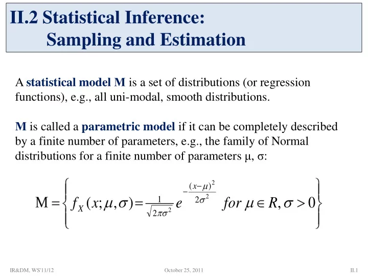
A statistical model Μ is a set of distributions (or regression functions), e.g., all uni-modal, smooth distributions. Μ is called a parametric model if it can be completely described by a finite number of parameters, e.g., the family of Normal distributions for a finite number of parameters μ, σ:

II.2 Statistical Inference: Sampling and Estimation

, ) , ; (

2 2 2

2 ) ( 2 1

R for e x f

x X

October 25, 2011 II.1 IR&DM, WS'11/12

Statistical Inference

Given a parametric model M and a sample X1,...,Xn, how do we infer (learn) the parameters of M? For multivariate models with observed variable X and „outcome (response)“ variable Y, this is called prediction

• r regression, for a discrete outcome variable this is also

called classification. r(x) = E[Y | X=x] is called the regression function.

October 25, 2011 II.2 IR&DM, WS'11/12

Idea of Sampling

Distribution X

(e.g., a population,

• bjects of interest)

Samples X1,…,Xn drawn from X

(e.g., people, objects)

Statistical Inference

What can we say about X based on X1,…,Xn?

Example:

Suppose we want to estimate the average salary of employees in German companies.  Sample 1: Suppose we look at n=200 top-paid CEOs of major banks.  Sample 2: Suppose we look at n=100 employees across all kinds of companies.

• Distrib. Param. Sample Param.

μX mean variance N size

n

X

2 X

S

2 X

October 25, 2011 II.3 IR&DM, WS'11/12

Basic Types of Statistical Inference

Given a set of iid. samples X1,...,Xn ~ X

• f an unknown distribution X.

e.g.: n single-coin-toss experiments X1,...,Xn ~ X: Bernoulli(p)

• Parameter Estimation

e.g.: - what is the parameter p of X: Bernoulli(p) ?

• what is E[X], the cdf FX of X, the pdf fX of X, etc.?
• Confidence Intervals

e.g.: give me all values C=(a,b) such that P(p C) ≥ 0.95

where a and b are derived from samples X1,...,Xn

• Hypothesis Testing

e.g.: H0 : p = 1/2 vs. H1 : p ≠ 1/2

October 25, 2011 II.4 IR&DM, WS'11/12

Statistical Estimators

A point estimator for a parameter of a prob. distribution X is a random variable derived from an iid. sample X1,...,Xn. Examples: Sample mean: Sample variance:

n i i

X n X

1

1 :

2 1 2

) ( 1 1 : X X n S

n i i X

An estimator for parameter is unbiased if E[ ] = ;

• therwise the estimator has bias E[ ] – .

An estimator on a sample of size n is consistent if 1 ] | ˆ [| lim any for P

n n

Sample mean and sample variance are unbiased and consistent estimators of μX and .

n

ˆ

n

ˆ

n

ˆ

n

ˆ

2 X

October 25, 2011 II.5 IR&DM, WS'11/12

Estimator Error

Let be an estimator for parameter over iid. samples X1, ...,Xn. The distribution of is called the sampling distribution. The standard error for is:

n

ˆ

n

ˆ

n

ˆ

The mean squared error (MSE) for is:

n

ˆ

2 n n

ˆ ˆ bias ( ) Var[ ]

Theorem: If bias 0 and se 0 then the estimator is consistent. The estimator is asymptotically Normal if converges in distribution to standard Normal N(0,1).

n

ˆ

n

ˆ ( ) / se

] ˆ [ ) ˆ (

n n

Var se

] ) ˆ [( ) ˆ (

2 n n

E MSE

October 25, 2011 II.6 IR&DM, WS'11/12

Types of Estimation

• Nonparametric Estimation

No assumptions about model M nor the parameters θ of the underlying distribution X “Plug-in estimators” (e.g. histograms) to approximate X

• Parametric Estimation (Inference)

Requires assumptions about model M and the parameters θ of the underlying distribution X Analytical or numerical methods for estimating θ Method-of-Moments estimator Maximum Likelihood estimator and Expectation Maximization (EM)

October 25, 2011 II.7 IR&DM, WS'11/12

Nonparametric Estimation

The empirical distribution function is the cdf that puts probability mass 1/n at each data point Xi:

n

ˆ F

n n i i 1

1 ˆ F ( x ) I( X x ) n A statistical functional (“statistics”) T(F) is any function over F, e.g., mean, variance, skewness, median, quantiles, correlation. The plug-in estimator of = T(F) is: n

n

ˆ ˆ T( F ) x X if x X if x X I with

i i i

1 ) (  Simply use instead of F to calculate the statistics T of interest.

n

ˆ F

October 25, 2011 II.8 IR&DM, WS'11/12

Histograms as Density Estimators

Instead of the full empirical distribution, often compact data synopses may be used, such as histograms where X1, ...,Xn are grouped into m cells (buckets) c1, ..., cm with bucket boundaries lb(ci) and ub(ci) s.t.

lb(c1) = , ub(cm ) = , ub(ci ) = lb(ci+1 ) for 1 i<m, and freqf (ci ) = freqF (ci ) =

Histograms provide a (discontinuous) density estimator.

Example:

X1= 1 X2= 1 X3= 2 X4= 2 X5= 2 X6= 3 … X20=7

x fX(x)

1 2 3 4 5 6 7

2/20 3/20 5/20 4/20 3/20 2/20 1/20

)) ( ) ( ( 1 ) ( ˆ

1 i n v v i n

c ub X c lb I n x f )) ( ( 1 ) ( ˆ

1 i n v v n

c ub X I n x F

65 . 3 20 1 7 20 2 6 20 3 5 20 4 4 20 5 3 20 3 2 20 2 1 ˆn

October 25, 2011 II.9 IR&DM, WS'11/12

Parametric Inference (1):

Method of Moments

Compute j-th moment: Method-of-moments estimators are usually consistent and asymptotically Normal, but may be biased.

n i j i j

X n

1

1 ˆ Suppose parameter θ = (θ1,…,θk ) has k components. dx x f x X E

X j j j j

) ( ] [ ) ( j-th sample moment: for 1 ≤ j ≤ k Estimate parameter by method-of-moments estimator s.t.

n

ˆ

and … … and (for the first k moments)

1 1

ˆ ) ˆ (

n 2 2

ˆ ) ˆ (

n k n k

ˆ ) ˆ (  Solve equation system with k equations and k unknowns.

October 25, 2011 II.10 IR&DM, WS'11/12

Parametric Inference (2):

Maximum Likelihood Estimators (MLE)

Let X1,...,Xn be iid. with pdf f(x;θ). Estimate parameter of a postulated distribution f(x; ) such that the likelihood that the sample values x1,...,xn are generated by this distribution is maximized. Maximum likelihood estimation: Maximize L(x1,...,xn; ) ≈ P[x1, ...,xn originate from f(x; )] Usually formulated as Ln( ) = ∏i f(Xi; ) Or (alternatively) Maximize ln( ) = log Ln( )

The value that maximizes Ln( ) is the MLE of .

If analytically untractable use numerical iteration methods

n

ˆ

October 25, 2011 II.11 IR&DM, WS'11/12

Simple Example for Maximum Likelihood Estimator

Given:

• Coin toss experiment (Bernoulli distribution) with

unknown parameter p for seeing heads, 1-p for tails

• Sample (data): h times head with n coin tosses

Want: Maximum likelihood estimation of p Let L(h, n, p) with h = ∑i Xi

h n h n i X X n i i

p p p p p X f

i i

) 1 ( ) 1 ( ) ; (

1 1 1

Maximize log-likelihood function: log L (h, n, p) n h p 1 ln p h n p h p L ) 1 log( ) ( ) log( p h n p h

October 25, 2011 II.12 IR&DM, WS'11/12

MLE for Parameters

• f Normal Distributions

n i x n n

i

e x x L

1 2 ) ( 2 1

2 2

2 1 ) , , ,..., (

n i 2 i 1

ln( L ) 1 2( x ) 2

2 1 2

1 2 4 2 2 n i i

) x ( n ) L ln(

n i i

x n

1

1 ˆ

2 1 2

) ˆ ( 1 ˆ

n i i

x n

October 25, 2011 II.13 IR&DM, WS'11/12

MLE Properties

Maximum Likelihood estimators are consistent, asymptotically Normal, and asymptotically optimal (i.e., efficient) in the following sense: Consider two estimators U and T which are asymptotically Normal. Let u2 and t2 denote the variances of the two Normal distributions to which U and T converge in probability. The asymptotic relative efficiency of U to T is ARE(U,T) := t2/u2 . Theorem: For an MLE and any other estimator the following inequality holds:

n

ˆ

n n n

ˆ ARE( , ) 1

That is, among all estimators MLE has the smallest variance.

October 25, 2011 II.14 IR&DM, WS'11/12

Bayesian Viewpoint of Parameter Estimation

• Assume prior distribution g( ) of parameter
• Choose statistical model (generative model) f (x | )

that reflects our beliefs about RV X

• Given RVs X1,...,Xn for the observed data,

the posterior distribution is h ( | x1,...,xn ) For X1= x1, ... ,Xn= xn the likelihood is which implies

(posterior is proportional to likelihood times prior)

MAP estimator (maximum a posteriori): Compute that maximizes h( | x1, …, xn ) given a prior for .

) ( ) , ... ( ~ ) ... | (

1 1

g x x L x x h

n n n i i i n i i n

g g x f x h x f x x L

1 ' 1 1

) ( ) ' ( ) ' | ( ) | ( ) | ( ) , ... (

October 25, 2011 II.15 IR&DM, WS'11/12

Analytically Non-tractable MLE for parameters

• f Multivariate Normal Mixture

) ,..., , ,..., , ,..., , (

1 1 1 k k k

x f   

k j x x j m j

j j T j

e

1 ) ( ) ( 2 1

1

) 2 ( 1

   

with expectation values and invertible, positive definite, symmetric m m covariance matrices

j



j k j j j j

x n

1

) , , (  

Maximize log-likelihood function:

n i k j j j i j n i i n

x n x P x x L

1 1 1 1

) , , ( log ] | [ log : ) , ,..., ( log     

Consider samples from a k-mixture of m-dimensional Normal distributions with the density (e.g. height and weight of males and females):

October 25, 2011 II.16 IR&DM, WS'11/12

Expectation-Maximization Method (EM)

] [ ] | , ... [ max arg ˆ

1

z Z P z Z X X J

n z

Key idea:

When L(X1,...,Xn, θ) (where the Xi and are possibly multivariate) is analytically intractable then

• introduce latent (i.e., hidden, invisible, missing) random variable(s) Z

such that

• the joint distribution J(X1,...,Xn, Z, ) of the “complete” data

is tractable (often with Z actually being multivariate: Z1,...,Zm)

• iteratively derive the expected complete-data likelihood by integrating J

and find best :

EZ|X, [J(X1,…,Xn, Z, )]

October 25, 2011 II.17 IR&DM, WS'11/12

EM Procedure

E step (expectation): estimate posterior probability of Z: P[Z | X1,…,Xn, (t)] assuming were known and equal to previous estimate (t), and compute EZ|X,θ(t) [log J(X1,…,Xn, Z, (t))] by integrating over values for Z Initialization: choose start estimate for (0)

(e.g., using Method-of-Moments estimator)

Iterate (t=0, 1, …) until convergence: M step (maximization, MLE step): Estimate (t+1) by maximizing

(t+1) = arg maxθ EZ|X,θ[log J(X1,…,Xn, Z, )]

 Convergence is guaranteed

(because the E step computes a lower bound of the true L function, and the M step yields monotonically non-decreasing likelihood),

but may result in local maximum of (log-)likelihood function

October 25, 2011 II.18 IR&DM, WS'11/12

EM Example for Multivariate Normal Mixture

i j ij ij i j n X Z

Z P Z x n Z X X J E ] 1 [ ) 1 | , ( log )] , , ,..., ( [log

1 , |

 Expectation step (E step):

( t ) ij ij i

h : P[ Z 1| x , ]

( t ) i j k ( t ) i l l 1

P[ x |n ( ) ] P[ x |n ( ) ]

Maximization step (M step):

n ij i i 1 j n ij i 1

h x : h

n T ij i j i j i 1 j n ij i 1

h ( x )( x ) : h

n n ij ij i 1 i 1 j k n ij j 1i 1

h h : n h Zij = 1 if ith data point Xi was generated by jth component, 0 otherwise

( t 1)

October 25, 2011 II.19 IR&DM, WS'11/12

See L. Wasserman, p.121 ff. for k=2, m=1

Confidence Intervals

Estimator T for an interval for parameter such that For the distribution of random variable X, a value x (0< <1) with is called a -quantile; the 0.5-quantile is called the median. For the Normal distribution N(0,1) the -quantile is denoted .

1 ] x X [ P ] x X [ P

1 ] a T a T [ P [T-a, T+a] is the confidence interval and 1– is the confidence level.

October 25, 2011 II.20 IR&DM, WS'11/12

 For a given a or α, find a value z of N(0,1) that denotes the [T-a, T+a] conf. interval

• r a corresponding -quantile for 1– .

Confidence Intervals for Expectations (1)

Let x1, ..., xn be a sample from a distribution with unknown expectation and known variance

2.

For sufficiently large n, the sample mean is N( ,

2/n) distributed

and is N(0,1) distributed:

X

n ) X (

1 ) ( 2 )) ( 1 ( ) ( ) ( ) ( ] ) ( [ z z z z z z n X z P ] [ n z X n z X P 1 ] [

2 / 1 2 / 1

n X n X P For confidence interval or confidence level 1- set

] , [ a X a X

n a : z ) , ( N

• f

quantile ) ( : z 1 2 1

then look up (z) to find 1–α

z a : n

then

October 25, 2011 II.21 IR&DM, WS'11/12

Confidence Intervals for Expectations (2)

Let X1, ..., Xn be an iid. sample from a distribution X with unknown expectation and unknown variance

2 and known sample variance S2.

For sufficiently large n, the random variable

S n X T ) ( :

has a t distribution (Student distribution) with n-1 degrees

• f freedom:

2 1 2 ,

1 1 2 2 1 ) (

n n T

n t n n n t f

with the Gamma function:

1

) ( x for dt t e x

x t

) ) x ( x ) x ( and ) ( properties the with ( 1 1 1

1

2 1 1 2 1 1

] n S t X n S t X [ P

/ , n / , n

October 25, 2011 II.22 IR&DM, WS'11/12

Summary of Section II.2

• Quality measures for statistical estimators
• Nonparametric vs. parametric estimation
• Histograms as generic (nonparametric) plug-in estimators
• Method-of-Moments estimator good initial guess but may be biased
• Maximum-Likelihood estimator & Expectation Maximization
• Confidence intervals for parameters

October 25, 2011 II.23 IR&DM, WS'11/12

Normal Distribution Table

October 25, 2011 II.24 IR&DM, WS'11/12

Student„s t Distribution Table

October 25, 2011 II.25 IR&DM, WS'11/12