How willing are you to be wrong? Type I and Type II Errors Type 1, - - PowerPoint PPT Presentation

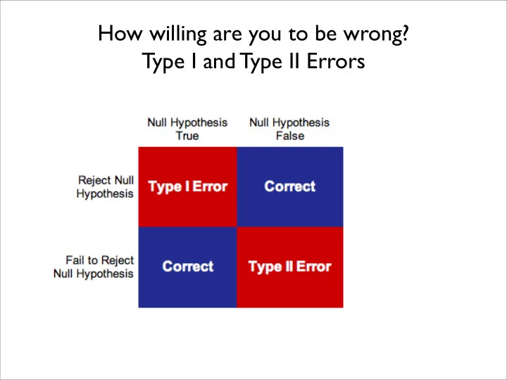
How willing are you to be wrong? Type I and Type II Errors

Type 1, Type II Errors and Power

Distribution of means for my data

Distribution of means for reference data a.k.a. Ho

5% of the data (the upper tail) is shaded, we will allow the distributions to overlap here and still reject Ho.

Type 1 and Type II Errors

• Our distributions overlap in the

Type I Error region, our “rejection region”. “If our

• bserved mean is > 1.16, we

reject the null hypothesis.”

• Thus we ALWAYS reject the null

hypothesis in this case, and our power is 100%

Type I and Type II Errors

Type I Error Our sample mean is 1.34. We reject Ho because 1.34 exceeds our critical value and is within the 0.05 tail of our reference

Our distributions match almost perfectly Ho=true. Yet, we will still reject Ho 5% of the time.

Type I and Type II Errors

Type II Error Our sample mean is 0.87. We do NOT reject Ho because 0.87 does not exceed

• ur critical value.
• As the true means of the

populations get closer...

As the distance between means shrinks, the power goes down because there is more overlap. Here, 50% of the means drawn from our population are less than the critical value, 1.16. So we can only detect a difference for 50%

• f our possible means.

How can we increase our power?

To increase power, increase ‘n’

Type I and Type II errors

Calculating Power

One-tailed test (right tailed)

X

U = µ0 + z σ

n

X

U our upper critical value, X-value here

µ0 mean for Ho

z

critical value of z given your choice of α

σ n

you should know this one by now but just in case, it’s the standard error of the mean

Calculating Power

One-tailed test (right tailed) Now find the z-value and beta (β)

z = X

U − x

σ n

X

U our upper critical value, X-value here

x the observed sample mean

For a right-tailed test find β β =P(z<z-critical) Power=1-β = P(z>z-critical)

β

Example

We have a sample of n=100 with a standard deviation of 3.6 and a mean of 17.9. We choose the following: α=0.05 Ho: μ=17.5 Ha: μ>17.5 What is the power of our z-test?

Calculating Power

X

U = µ0 + z σ

n

X

U =17.5 +1.65 3.6

10

X

U =18.1

z = X

U − x

σ n

z = 18.1−17.9 0.36

Probability of getting a value to the RIGHT of 0.54 p=0.2946 = power (1-β)

z = 0.54

β β β

Increasing power

• Increase alpha (α)
• Increase “n”
• Decrease standard deviation
• Use a 1-tailed test

JMP time