
SLIDE 1
1
CS 3343 Analysis of Algorithms 1 2/24/09
CS 3343 -- Spring 2009
Sorting
Carola Wenk Slides courtesy of Charles Leiserson with small changes by Carola Wenk
CS 3343 Analysis of Algorithms 2 2/24/09
How fast can we sort?
All the sorting algorithms we have seen so far are comparison sorts: only use comparisons to determine the relative order of elements.
- E.g., insertion sort, merge sort, quicksort,
heapsort. The best worst-case running time that we’ve seen for comparison sorting is O(nlogn). Is O(nlogn) the best we can do? Decision trees can help us answer this question.
CS 3343 Analysis of Algorithms 3 2/24/09
Decision-tree model
A decision tree models the execution of any comparison sorting algorithm:
- One tree per input size n.
- The tree contains all possible comparisons (= if-branches)
that could be executed for any input of size n.
- The tree contains all comparisons along all possible
instruction traces (= control flows) for all inputs of size n.
- For one input, only one path to a leaf is executed.
- Running time = length of the path taken.
- Worst-case running time = height of tree.
CS 3343 Analysis of Algorithms 4 2/24/09
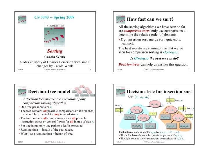
Decision-tree for insertion sort
a1:a2 a1:a2 a2:a3 a2:a3 a1a2a3 a1a2a3 a1:a3 a1:a3 a1a3a2 a1a3a2 a3a1a2 a3a1a2 a1:a3 a1:a3 a2a1a3 a2a1a3 a2:a3 a2:a3 a2a3a1 a2a3a1 a3a2a1 a3a2a1
Each internal node is labeled ai:aj for i, j ∈ {1, 2,…, n}.
- The left subtree shows subsequent comparisons if ai < aj.
- The right subtree shows subsequent comparisons if ai ≥ aj.
Sort 〈a1, a2, a3〉
< < < < < ≥ ≥ ≥ ≥ ≥
a1 a2 a3 a1 a2 a3 a2 a1 a3 i j i j i j a2 a1 a3 i j a1 a2 a3 i j insert a3 insert a3 insert a2