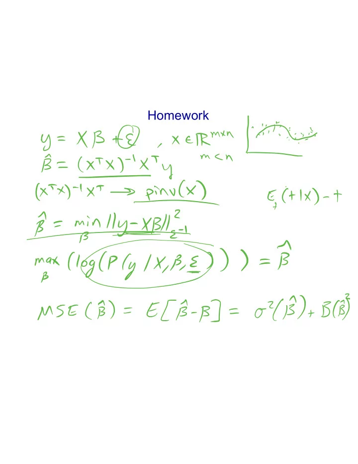
SLIDE 1
Homework
SLIDE 2
Homework
SLIDE 3
Lecture 7: Linear Classification Methods
Final projects? Groups Topics Proposal week 5 Lecture 20 is poster session, Jacobs Hall Lobby, snacks Final report 15 June.
SLIDE 4
What is “linear” classification?
Classification is intrinsically non-linear It puts non-identical things in the same class, so a difference in input vector sometimes causes zero change in the answer “Linear classification” means that the part that adapts is linear The adaptive part is followed by a fixed non-linearity. It may be preceded by a fixed non-linearity (e.g. nonlinear basis functions).
)) ( ( , ) ( x x w x y f Decision w y
T
= + =
fixed non-linear function adaptive linear function 0.5 1
z y
SLIDE 5
Representing the target values for classification
For two classes, we use a single valued output that has target values 1 for the “positive” class and 0 (or -1) for the other class For probabilistic class labels the target value can then be P(t=1) and the model output can also represent P(y=1). For N classes we often use a vector of N target values containing a single 1 for the correct class and zeros elsewhere. For probabilistic labels we can then use a vector of class probabilities as the target vector.
SLIDE 6 Three approaches to classification
Use discriminant functions directly without probabilities: Convert input vector into real values. A simple operation (like thresholding) can get the class.
Choose real values to maximize the useable information about the class label that is in the real value.
Infer conditional class probabilities: Compute the conditional probability of each class.
Then make a decision that minimizes some loss function
Compare the probability of the input under separate, class- specific, generative models. E.g. fit a multivariate Gaussian to the input vectors of each class and see which Gaussian makes a test data vector most
- probable. (Is this the best bet?)
) | ( x
k
C class p =
SLIDE 7
The planar decision surface in data-space for the simple linear discriminant function:
0 ³
+ w
Tx
w
X on plane => y=0 => Distance from plane Discriminant functions
SLIDE 8
Discriminant functions for N>2 classes
One possibility is to use N two-way discriminant functions. Each function discriminates one class from the rest. Another possibility is to use N(N-1)/2 two-way discriminant functions Each function discriminates between two particular classes. Both these methods have problems More than one good answer Two-way preferences need not be transitive!
SLIDE 9 A simple solution (4.1.2)
Use N discriminant functions, and pick the max.
This is guaranteed to give consistent and convex decision regions if y is linear.
( ) ( )
B A j B A k B j B k A j A k
y y that positive for implies y y and y y x x x x x x x x ) 1 ( ) 1 ( ) ( ) ( ) ( ) ( ) ( a a a a a
>
> > ... , ,
k j i
y y y
Decision boundary?
SLIDE 10 Maximum Likelihood and Least Squares (from lecture 3)
Computing the gradient and setting it to zero yields Solving for w, where
The Moore-Penrose pseudo-inverse, .
SLIDE 11 LSQ for classification
Each class Ck is described by its own linear model so that yk(x) = wT
k x + wk0
(4.13) where k = 1, . . . , K. We can conveniently group these together using vector nota- tion so that y(x) = WT x (4.14)
Consider a training set {"#, $#}, ' = 1 …N Define X and T
XT X)−1 XTT = X†T (4.16)
And prediction
WT x = TT
(4.17)
SLIDE 12
Using “least squares” for classification
It does not work as well as better methods, but it is easy: It reduces classification to least squares regression.
logistic regression least squares regression
SLIDE 13
PCA don’t work well
SLIDE 14
picture showing the advantage of Fisher’s linear discriminant
When projected onto the line joining the class means, the classes are not well separated. Fisher chooses a direction that makes the projected classes much tighter, even though their projected means are less far apart.
SLIDE 15 Math of Fisher’s linear discriminants
What linear transformation is best for discrimination? The projection onto the vector separating the class means seems sensible: But we also want small variance within each class: Fisher’s objective function is:
x wT y =
1 2
m m w
) ( ) (
2 2 2 1 2 1
2 1
m y s m y s
C n n C n n
å å
e e 2 2 2 1 2 1 2
) ( ) ( s s m m J +
w
between within
SLIDE 16 ) ( : ) ( ) ( ) ( ) ( ) ( ) ( ) ( ) (
1 2 1 2 2 1 1 1 2 1 2 2 2 2 1 2 1 2
2 1
m m S w m x m x m x m x S m m m m S w S w w S w w
= +
Î
å å
W C n T n n C n T n n W T B W T B T
solution Optimal s s m m J
More math of Fisher’s linear discriminants
SLIDE 17
We have probalistic classification!
SLIDE 18 Probabilistic Generative Models for Discrimination (Bishop p 196)
Use a generative model of the input vectors for each class, and see which model makes a test input vector most probable. The posterior probability of class 1 is:
) | ( 1 ) | ( ln ) | ( ) ( ) | ( ) ( ln 1 1 ) | ( ) ( ) | ( ) ( ) | ( ) ( ) | (
1 1 1 1 1 1 1 1 1
x x x x x x x x C p C p C p C p C p C p z where e C p C p C p C p C p C p C p
z
= + = + =
- z is called the logit and is
given by the log odds
SLIDE 19 An example for continuous inputs
Assume input vectors for each class are Gaussian, all classes have the same covariance matrix. For two classes, C1 and C0, the posterior is a logistic:
{ }
) ( ) ( exp ) | (
1 2 1 k T k k
a C p µ x µ x x
( ) ( ln ) ( ) ( ) | (
1 1 2 1 1 1 1 2 1 1 1 1
C p C p w w C p
T T T
+ +
+ =
Σ µ µ Σ µ µ µ Σ w x w x s
inverse covariance matrix normalizing constant
SLIDE 20
! = #$ % &|() % () % &|(* % (*
SLIDE 21 The role of the inverse covariance matrix
If the Gaussian is spherical no need to worry about the covariance matrix. So, start by transforming the data space to make the Gaussian spherical This is called “whitening” the data. It pre-multiplies by the matrix square root of the inverse covariance matrix. In transformed space, the weight vector is the difference between transformed means.
aff T aff aff aff T
for gives and as for value same the gives x w x Σ x µ Σ µ Σ w x w µ µ Σ w
2 1 2 1 2 1
1 1 1
: ) (
SLIDE 22
The posterior when the covariance matrices are different for different classes (Bishop Fig )
The decision surface is planar when the covariance matrices are the same and quadratic when not.
SLIDE 23
Bernoulli distribution Random variable ! ∈ 0,1
Coin flipping: heads=1, tails=0 Bernoulli Distribution
ML for Bernoulli Given:
SLIDE 24 The logistic function
The output is a smooth function
- f the inputs and the weights.
) 1 ( ) (
1 1
y y dz dy w x z x w z z e z y w z
i i i i T
= ¶ ¶ = ¶ ¶
= = + = s x w
0.5 1
z y
Its odd to express it in terms of y.
SLIDE 25
Logistic regression (Bishop 205)
! "# $ = &(()$) Observations Likelihood 2 = &(()$) ! 2 $, ( = ! 4 $, ( = Log-likelihood Minimize –log like Derivative ∇(C( =
C( = −EF(! 4 $, ( )=
SLIDE 26 Logistic regression (page 205)
When there are only two classes we can model the conditional probability of the positive class as If we use the right error function, something nice happens: The gradient of the logistic and the gradient of the error function cancel each other:
) exp( 1 1 ) ( ) ( ) | (
1
z z where w C p
T
= + = s s x w x
n n N n n
t y E p E x w w t w ) ( ) ( ), | ( ln ) (
1
Ñ
å
=