High-speed cryptography, Cryptographers part 3: more - - PowerPoint PPT Presentation

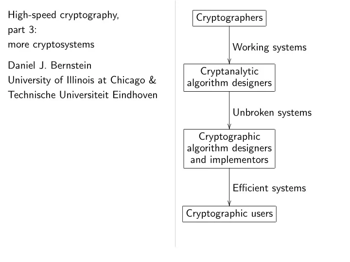
High-speed cryptography, part 3: more cryptosystems Daniel J. Bernstein University of Illinois at Chicago & Technische Universiteit Eindhoven Cryptographers Working systems

• Cryptanalytic

algorithm designers Unbroken systems

• Cryptographic

algorithm designers and implementors Efficient systems

• Cryptographic users

High-speed cryptography, 3: cryptosystems

• J. Bernstein

University of Illinois at Chicago & echnische Universiteit Eindhoven Cryptographers Working systems

• Cryptanalytic

algorithm designers Unbroken systems

• Cryptographic

algorithm designers and implementors Efficient systems

• Cryptographic users
• 1. Working

Fundamental cryptographers: How can sign, verify Many answ DES, Triple RSA, McEliece Merkle hash-tree Merkle–Hellman encryption, class-group ECDSA,

cryptography, cryptosystems Bernstein Illinois at Chicago & Universiteit Eindhoven Cryptographers Working systems

• Cryptanalytic

algorithm designers Unbroken systems

• Cryptographic

algorithm designers and implementors Efficient systems

• Cryptographic users
• 1. Working systems

Fundamental question cryptographers: How can we encrypt, sign, verify, etc.? Many answers: DES, Triple DES, RSA, McEliece encryption, Merkle hash-tree signatures, Merkle–Hellman knapsack encryption, Buchmann–Williams class-group encryption, ECDSA, HFEv, NTRU,

Chicago & Eindhoven Cryptographers Working systems

• Cryptanalytic

algorithm designers Unbroken systems

• Cryptographic

algorithm designers and implementors Efficient systems

• Cryptographic users
• 1. Working systems

Fundamental question for cryptographers: How can we encrypt, decrypt, sign, verify, etc.? Many answers: DES, Triple DES, FEAL-4, AES, RSA, McEliece encryption, Merkle hash-tree signatures, Merkle–Hellman knapsack encryption, Buchmann–Williams class-group encryption, ECDSA, HFEv, NTRU, et

Cryptographers Working systems

• Cryptanalytic

algorithm designers Unbroken systems

• Cryptographic

algorithm designers and implementors Efficient systems

• Cryptographic users
• 1. Working systems

Fundamental question for cryptographers: How can we encrypt, decrypt, sign, verify, etc.? Many answers: DES, Triple DES, FEAL-4, AES, RSA, McEliece encryption, Merkle hash-tree signatures, Merkle–Hellman knapsack encryption, Buchmann–Williams class-group encryption, ECDSA, HFEv, NTRU, et al.

Cryptographers Working systems

• Cryptanalytic

rithm designers Unbroken systems

• Cryptographic

rithm designers implementors Efficient systems

• Cryptographic users
• 1. Working systems

Fundamental question for cryptographers: How can we encrypt, decrypt, sign, verify, etc.? Many answers: DES, Triple DES, FEAL-4, AES, RSA, McEliece encryption, Merkle hash-tree signatures, Merkle–Hellman knapsack encryption, Buchmann–Williams class-group encryption, ECDSA, HFEv, NTRU, et al.

• 2. Unbrok

Fundamental pre-quantum What can using ❁2❜

• n a classical

Fundamental post-quantum What can using ❁2❜

• n a quantum

Goal: identify not break ❁ ❜

Cryptographers rking systems Cryptanalytic designers roken systems Cryptographic designers implementors Efficient systems users

• 1. Working systems

Fundamental question for cryptographers: How can we encrypt, decrypt, sign, verify, etc.? Many answers: DES, Triple DES, FEAL-4, AES, RSA, McEliece encryption, Merkle hash-tree signatures, Merkle–Hellman knapsack encryption, Buchmann–Williams class-group encryption, ECDSA, HFEv, NTRU, et al.

• 2. Unbroken systems

Fundamental question pre-quantum cryptanalysts: What can an attack using ❁2❜ operations

• n a classical computer?

Fundamental question post-quantum cryptanalysts: What can an attack using ❁2❜ operations

• n a quantum computer?

Goal: identify systems not breakable in ❁ ❜

systems systems ms

• 1. Working systems

Fundamental question for cryptographers: How can we encrypt, decrypt, sign, verify, etc.? Many answers: DES, Triple DES, FEAL-4, AES, RSA, McEliece encryption, Merkle hash-tree signatures, Merkle–Hellman knapsack encryption, Buchmann–Williams class-group encryption, ECDSA, HFEv, NTRU, et al.

• 2. Unbroken systems

Fundamental question for pre-quantum cryptanalysts: What can an attacker do using ❁2❜ operations

• n a classical computer?

Fundamental question for post-quantum cryptanalysts: What can an attacker do using ❁2❜ operations

• n a quantum computer?

Goal: identify systems that a not breakable in ❁2❜ operations.

• 1. Working systems

Fundamental question for cryptographers: How can we encrypt, decrypt, sign, verify, etc.? Many answers: DES, Triple DES, FEAL-4, AES, RSA, McEliece encryption, Merkle hash-tree signatures, Merkle–Hellman knapsack encryption, Buchmann–Williams class-group encryption, ECDSA, HFEv, NTRU, et al.

• 2. Unbroken systems

Fundamental question for pre-quantum cryptanalysts: What can an attacker do using ❁2❜ operations

• n a classical computer?

Fundamental question for post-quantum cryptanalysts: What can an attacker do using ❁2❜ operations

• n a quantum computer?

Goal: identify systems that are not breakable in ❁2❜ operations.

rking systems undamental question for cryptographers: can we encrypt, decrypt, verify, etc.? answers: Triple DES, FEAL-4, AES, McEliece encryption, hash-tree signatures, Merkle–Hellman knapsack encryption, Buchmann–Williams class-group encryption, ECDSA, HFEv, NTRU, et al.

• 2. Unbroken systems

Fundamental question for pre-quantum cryptanalysts: What can an attacker do using ❁2❜ operations

• n a classical computer?

Fundamental question for post-quantum cryptanalysts: What can an attacker do using ❁2❜ operations

• n a quantum computer?

Goal: identify systems that are not breakable in ❁2❜ operations. Examples Schroepp mentioned factors ♣q ♣❀ q (2 + ♦(1))

♣q

❂

♣q

❂

simple op To push

❜

must cho ♣q (0✿5 + ♦(1))❜ ❂ ❜ Note 1: Note 2: ♦ about, e.g., ❜ Today: fo

systems uestion for encrypt, decrypt, DES, FEAL-4, AES, encryption, signatures, knapsack Buchmann–Williams encryption,

, NTRU, et al.

• 2. Unbroken systems

Fundamental question for pre-quantum cryptanalysts: What can an attacker do using ❁2❜ operations

• n a classical computer?

Fundamental question for post-quantum cryptanalysts: What can an attacker do using ❁2❜ operations

• n a quantum computer?

Goal: identify systems that are not breakable in ❁2❜ operations. Examples of RSA cryptanalysis: Schroeppel’s “linea mentioned in 1978 factors ♣q into ♣❀ q (2 + ♦(1))(lg ♣q)1❂2(lg

♣q

❂

simple operations (conjec To push this beyond

❜

must choose ♣q to (0✿5 + ♦(1))❜2❂lg ❜ Note 1: lg = log2. Note 2: ♦(1) says about, e.g., ❜ = 128. Today: focus on asymptotics.

decrypt, FEAL-4, AES, encryption, signatures, Buchmann–Williams

• et al.
• 2. Unbroken systems

Fundamental question for pre-quantum cryptanalysts: What can an attacker do using ❁2❜ operations

• n a classical computer?

Fundamental question for post-quantum cryptanalysts: What can an attacker do using ❁2❜ operations

• n a quantum computer?

Goal: identify systems that are not breakable in ❁2❜ operations. Examples of RSA cryptanalysis: Schroeppel’s “linear sieve”, mentioned in 1978 RSA pap factors ♣q into ♣❀ q using (2 + ♦(1))(lg ♣q)1❂2(lg lg ♣q)1❂2 simple operations (conjecturally). To push this beyond 2❜, must choose ♣q to have at least (0✿5 + ♦(1))❜2❂lg ❜ bits. Note 1: lg = log2. Note 2: ♦(1) says nothing about, e.g., ❜ = 128. Today: focus on asymptotics.

• 2. Unbroken systems

Fundamental question for pre-quantum cryptanalysts: What can an attacker do using ❁2❜ operations

• n a classical computer?

Fundamental question for post-quantum cryptanalysts: What can an attacker do using ❁2❜ operations

• n a quantum computer?

Goal: identify systems that are not breakable in ❁2❜ operations. Examples of RSA cryptanalysis: Schroeppel’s “linear sieve”, mentioned in 1978 RSA paper, factors ♣q into ♣❀ q using (2 + ♦(1))(lg ♣q)1❂2(lg lg ♣q)1❂2 simple operations (conjecturally). To push this beyond 2❜, must choose ♣q to have at least (0✿5 + ♦(1))❜2❂lg ❜ bits. Note 1: lg = log2. Note 2: ♦(1) says nothing about, e.g., ❜ = 128. Today: focus on asymptotics.

Unbroken systems undamental question for re-quantum cryptanalysts: can an attacker do ❁2❜ operations classical computer? undamental question for

• st-quantum cryptanalysts:

can an attacker do ❁2❜ operations quantum computer? identify systems that are reakable in ❁2❜ operations. Examples of RSA cryptanalysis: Schroeppel’s “linear sieve”, mentioned in 1978 RSA paper, factors ♣q into ♣❀ q using (2 + ♦(1))(lg ♣q)1❂2(lg lg ♣q)1❂2 simple operations (conjecturally). To push this beyond 2❜, must choose ♣q to have at least (0✿5 + ♦(1))❜2❂lg ❜ bits. Note 1: lg = log2. Note 2: ♦(1) says nothing about, e.g., ❜ = 128. Today: focus on asymptotics. 1993 Buhler–Lenstra–P generalizing “number-field factors ♣q ♣❀ q (3✿79 ✿ ✿ ✿ ♦

♣q

❂

♣q

❂

simple op To push

❜

must cho ♣q (0✿015 ✿ ✿ ✿ ♦ ❜ ❂ ❜ Subsequent 3✿73 ✿ ✿ ✿; ♦ But can that 2(lg ♣q

❂ ♦

—for cla

systems uestion for cryptanalysts: attacker do ❁ ❜ erations computer? uestion for cryptanalysts: attacker do ❁ ❜ erations computer? systems that are ❁2❜ operations. Examples of RSA cryptanalysis: Schroeppel’s “linear sieve”, mentioned in 1978 RSA paper, factors ♣q into ♣❀ q using (2 + ♦(1))(lg ♣q)1❂2(lg lg ♣q)1❂2 simple operations (conjecturally). To push this beyond 2❜, must choose ♣q to have at least (0✿5 + ♦(1))❜2❂lg ❜ bits. Note 1: lg = log2. Note 2: ♦(1) says nothing about, e.g., ❜ = 128. Today: focus on asymptotics. 1993 Buhler–Lenstra–P generalizing 1988 P “number-field sieve”, factors ♣q into ♣❀ q (3✿79 ✿ ✿ ✿ + ♦(1))(lg ♣q

❂

♣q

❂

simple operations (conjec To push this beyond

❜

must choose ♣q to (0✿015 ✿ ✿ ✿ + ♦(1))❜ ❂ ❜ Subsequent improveme 3✿73 ✿ ✿ ✿; details of ♦ But can reasonably that 2(lg ♣q)1❂3+♦(1) —for classical computers.

cryptanalysts: ❁ ❜ cryptanalysts: ❁ ❜ that are ❁ ❜ erations. Examples of RSA cryptanalysis: Schroeppel’s “linear sieve”, mentioned in 1978 RSA paper, factors ♣q into ♣❀ q using (2 + ♦(1))(lg ♣q)1❂2(lg lg ♣q)1❂2 simple operations (conjecturally). To push this beyond 2❜, must choose ♣q to have at least (0✿5 + ♦(1))❜2❂lg ❜ bits. Note 1: lg = log2. Note 2: ♦(1) says nothing about, e.g., ❜ = 128. Today: focus on asymptotics. 1993 Buhler–Lenstra–Pomera generalizing 1988 Pollard “number-field sieve”, factors ♣q into ♣❀ q using (3✿79 ✿ ✿ ✿ + ♦(1))(lg ♣q)1❂3(lg lg ♣q

❂

simple operations (conjecturally). To push this beyond 2❜, must choose ♣q to have at least (0✿015 ✿ ✿ ✿ + ♦(1))❜3❂(lg ❜)2 bits. Subsequent improvements: 3✿73 ✿ ✿ ✿; details of ♦(1). But can reasonably conjecture that 2(lg ♣q)1❂3+♦(1) is optimal —for classical computers.

Examples of RSA cryptanalysis: Schroeppel’s “linear sieve”, mentioned in 1978 RSA paper, factors ♣q into ♣❀ q using (2 + ♦(1))(lg ♣q)1❂2(lg lg ♣q)1❂2 simple operations (conjecturally). To push this beyond 2❜, must choose ♣q to have at least (0✿5 + ♦(1))❜2❂lg ❜ bits. Note 1: lg = log2. Note 2: ♦(1) says nothing about, e.g., ❜ = 128. Today: focus on asymptotics. 1993 Buhler–Lenstra–Pomerance, generalizing 1988 Pollard “number-field sieve”, factors ♣q into ♣❀ q using (3✿79 ✿ ✿ ✿ + ♦(1))(lg ♣q)1❂3(lg lg ♣q)2❂3 simple operations (conjecturally). To push this beyond 2❜, must choose ♣q to have at least (0✿015 ✿ ✿ ✿ + ♦(1))❜3❂(lg ❜)2 bits. Subsequent improvements: 3✿73 ✿ ✿ ✿; details of ♦(1). But can reasonably conjecture that 2(lg ♣q)1❂3+♦(1) is optimal —for classical computers.

Examples of RSA cryptanalysis: eppel’s “linear sieve”, mentioned in 1978 RSA paper, ♣q into ♣❀ q using ♦(1))(lg ♣q)1❂2(lg lg ♣q)1❂2

• perations (conjecturally).

push this beyond 2❜, choose ♣q to have at least ✿ ♦(1))❜2❂lg ❜ bits. 1: lg = log2. 2: ♦(1) says nothing e.g., ❜ = 128. y: focus on asymptotics. 1993 Buhler–Lenstra–Pomerance, generalizing 1988 Pollard “number-field sieve”, factors ♣q into ♣❀ q using (3✿79 ✿ ✿ ✿ + ♦(1))(lg ♣q)1❂3(lg lg ♣q)2❂3 simple operations (conjecturally). To push this beyond 2❜, must choose ♣q to have at least (0✿015 ✿ ✿ ✿ + ♦(1))❜3❂(lg ❜)2 bits. Subsequent improvements: 3✿73 ✿ ✿ ✿; details of ♦(1). But can reasonably conjecture that 2(lg ♣q)1❂3+♦(1) is optimal —for classical computers. Cryptographic pre-quantum Triple DES ❜ ✔ AES-256 ❜ ✔ RSA with ❜

♦

McEliece ❜1+♦(1), with “strong” ❜

♦

BW with ❜

♦

bit discriminant, “strong” ❜

♦

HFEv with ❜

♦

NTRU with ❜

♦

RSA cryptanalysis: “linear sieve”, 1978 RSA paper, ♣q ♣❀ q using ♦

♣q

❂2(lg lg ♣q)1❂2

erations (conjecturally).

• nd 2❜,

♣q to have at least ✿ ♦ ❜ ❂lg ❜ bits.

2.

♦ ys nothing ❜ 128. asymptotics. 1993 Buhler–Lenstra–Pomerance, generalizing 1988 Pollard “number-field sieve”, factors ♣q into ♣❀ q using (3✿79 ✿ ✿ ✿ + ♦(1))(lg ♣q)1❂3(lg lg ♣q)2❂3 simple operations (conjecturally). To push this beyond 2❜, must choose ♣q to have at least (0✿015 ✿ ✿ ✿ + ♦(1))❜3❂(lg ❜)2 bits. Subsequent improvements: 3✿73 ✿ ✿ ✿; details of ♦(1). But can reasonably conjecture that 2(lg ♣q)1❂3+♦(1) is optimal —for classical computers. Cryptographic systems pre-quantum cryptanalysis: Triple DES (for ❜ ✔ AES-256 (for ❜ ✔ 256), RSA with ❜3+♦(1)-bit McEliece with code ❜1+♦(1), Merkle signatures with “strong” ❜1+♦ BW with “strong” ❜

♦

bit discriminant, ECDSA “strong” ❜1+♦(1)-bit HFEv with ❜1+♦(1) NTRU with ❜1+♦(1)

cryptanalysis: sieve”, paper, ♣q ♣❀ q ♦

♣q

❂

♣q

❂2

turally).

❜

♣q at least ✿ ♦ ❜ ❂ ❜ ♦ ❜ asymptotics. 1993 Buhler–Lenstra–Pomerance, generalizing 1988 Pollard “number-field sieve”, factors ♣q into ♣❀ q using (3✿79 ✿ ✿ ✿ + ♦(1))(lg ♣q)1❂3(lg lg ♣q)2❂3 simple operations (conjecturally). To push this beyond 2❜, must choose ♣q to have at least (0✿015 ✿ ✿ ✿ + ♦(1))❜3❂(lg ❜)2 bits. Subsequent improvements: 3✿73 ✿ ✿ ✿; details of ♦(1). But can reasonably conjecture that 2(lg ♣q)1❂3+♦(1) is optimal —for classical computers. Cryptographic systems surviving pre-quantum cryptanalysis: Triple DES (for ❜ ✔ 112), AES-256 (for ❜ ✔ 256), RSA with ❜3+♦(1)-bit modulus, McEliece with code length ❜1+♦(1), Merkle signatures with “strong” ❜1+♦(1)-bit hash, BW with “strong” ❜2+♦(1)- bit discriminant, ECDSA with “strong” ❜1+♦(1)-bit curve, HFEv with ❜1+♦(1) polynomials, NTRU with ❜1+♦(1) bits, et al.

1993 Buhler–Lenstra–Pomerance, generalizing 1988 Pollard “number-field sieve”, factors ♣q into ♣❀ q using (3✿79 ✿ ✿ ✿ + ♦(1))(lg ♣q)1❂3(lg lg ♣q)2❂3 simple operations (conjecturally). To push this beyond 2❜, must choose ♣q to have at least (0✿015 ✿ ✿ ✿ + ♦(1))❜3❂(lg ❜)2 bits. Subsequent improvements: 3✿73 ✿ ✿ ✿; details of ♦(1). But can reasonably conjecture that 2(lg ♣q)1❂3+♦(1) is optimal —for classical computers. Cryptographic systems surviving pre-quantum cryptanalysis: Triple DES (for ❜ ✔ 112), AES-256 (for ❜ ✔ 256), RSA with ❜3+♦(1)-bit modulus, McEliece with code length ❜1+♦(1), Merkle signatures with “strong” ❜1+♦(1)-bit hash, BW with “strong” ❜2+♦(1)- bit discriminant, ECDSA with “strong” ❜1+♦(1)-bit curve, HFEv with ❜1+♦(1) polynomials, NTRU with ❜1+♦(1) bits, et al.

Buhler–Lenstra–Pomerance, generalizing 1988 Pollard er-field sieve”, ♣q into ♣❀ q using ✿ ✿ ✿ ✿ + ♦(1))(lg ♣q)1❂3(lg lg ♣q)2❂3

• perations (conjecturally).

push this beyond 2❜, choose ♣q to have at least ✿ ✿ ✿ ✿ + ♦(1))❜3❂(lg ❜)2 bits. Subsequent improvements: ✿ ✿ ✿ ✿; details of ♦(1). can reasonably conjecture

(lg ♣q)1❂3+♦(1) is optimal

classical computers. Cryptographic systems surviving pre-quantum cryptanalysis: Triple DES (for ❜ ✔ 112), AES-256 (for ❜ ✔ 256), RSA with ❜3+♦(1)-bit modulus, McEliece with code length ❜1+♦(1), Merkle signatures with “strong” ❜1+♦(1)-bit hash, BW with “strong” ❜2+♦(1)- bit discriminant, ECDSA with “strong” ❜1+♦(1)-bit curve, HFEv with ❜1+♦(1) polynomials, NTRU with ❜1+♦(1) bits, et al. Typical algo pre-quantum NFS, ✚, Post-quantum have all plus quantum Spectacula 1994 Sho ♣q ♣❀ q using (lg ♣q

♦

simple quantum To push

❜

must cho ♣q 2(0✿5+♦(1))❜

Buhler–Lenstra–Pomerance, 1988 Pollard sieve”, ♣q ♣❀ q using ✿ ✿ ✿ ✿ ♦

(lg ♣q)1❂3(lg lg ♣q)2❂3

erations (conjecturally).

• nd 2❜,

♣q to have at least ✿ ✿ ✿ ✿ ♦(1))❜3❂(lg ❜)2 bits. rovements: ✿ ✿ ✿ ✿

• f ♦(1).

reasonably conjecture

♣q

❂ ♦(1) is optimal

computers. Cryptographic systems surviving pre-quantum cryptanalysis: Triple DES (for ❜ ✔ 112), AES-256 (for ❜ ✔ 256), RSA with ❜3+♦(1)-bit modulus, McEliece with code length ❜1+♦(1), Merkle signatures with “strong” ❜1+♦(1)-bit hash, BW with “strong” ❜2+♦(1)- bit discriminant, ECDSA with “strong” ❜1+♦(1)-bit curve, HFEv with ❜1+♦(1) polynomials, NTRU with ❜1+♦(1) bits, et al. Typical algorithmic pre-quantum cryptanalysts: NFS, ✚, ISD, LLL, Post-quantum cryptanalysts have all the same to plus quantum algo Spectacular example: 1994 Shor factors ♣q ♣❀ q using (lg ♣q)2+♦(1) simple quantum op To push this beyond

❜

must choose ♣q to 2(0✿5+♦(1))❜ bits. Yik

• merance,

♣q ♣❀ q ✿ ✿ ✿ ✿ ♦

♣q

❂

lg ♣q)2❂3

turally).

❜

♣q at least ✿ ✿ ✿ ✿ ♦ ❜ ❂ ❜ bits. nts: ✿ ✿ ✿ ✿ ♦ conjecture

♣q

❂ ♦

• ptimal

Cryptographic systems surviving pre-quantum cryptanalysis: Triple DES (for ❜ ✔ 112), AES-256 (for ❜ ✔ 256), RSA with ❜3+♦(1)-bit modulus, McEliece with code length ❜1+♦(1), Merkle signatures with “strong” ❜1+♦(1)-bit hash, BW with “strong” ❜2+♦(1)- bit discriminant, ECDSA with “strong” ❜1+♦(1)-bit curve, HFEv with ❜1+♦(1) polynomials, NTRU with ❜1+♦(1) bits, et al. Typical algorithmic tools for pre-quantum cryptanalysts: NFS, ✚, ISD, LLL, F4, XL, et Post-quantum cryptanalysts have all the same tools plus quantum algorithms. Spectacular example: 1994 Shor factors ♣q into ♣❀ q using (lg ♣q)2+♦(1) simple quantum operations. To push this beyond 2❜, must choose ♣q to have at least 2(0✿5+♦(1))❜ bits. Yikes.

Cryptographic systems surviving pre-quantum cryptanalysis: Triple DES (for ❜ ✔ 112), AES-256 (for ❜ ✔ 256), RSA with ❜3+♦(1)-bit modulus, McEliece with code length ❜1+♦(1), Merkle signatures with “strong” ❜1+♦(1)-bit hash, BW with “strong” ❜2+♦(1)- bit discriminant, ECDSA with “strong” ❜1+♦(1)-bit curve, HFEv with ❜1+♦(1) polynomials, NTRU with ❜1+♦(1) bits, et al. Typical algorithmic tools for pre-quantum cryptanalysts: NFS, ✚, ISD, LLL, F4, XL, et al. Post-quantum cryptanalysts have all the same tools plus quantum algorithms. Spectacular example: 1994 Shor factors ♣q into ♣❀ q using (lg ♣q)2+♦(1) simple quantum operations. To push this beyond 2❜, must choose ♣q to have at least 2(0✿5+♦(1))❜ bits. Yikes.

Cryptographic systems surviving re-quantum cryptanalysis: DES (for ❜ ✔ 112), AES-256 (for ❜ ✔ 256), with ❜3+♦(1)-bit modulus, McEliece with code length ❜

♦

, Merkle signatures “strong” ❜1+♦(1)-bit hash, with “strong” ❜2+♦(1)- discriminant, ECDSA with “strong” ❜1+♦(1)-bit curve,

with ❜1+♦(1) polynomials,

with ❜1+♦(1) bits, et al. Typical algorithmic tools for pre-quantum cryptanalysts: NFS, ✚, ISD, LLL, F4, XL, et al. Post-quantum cryptanalysts have all the same tools plus quantum algorithms. Spectacular example: 1994 Shor factors ♣q into ♣❀ q using (lg ♣q)2+♦(1) simple quantum operations. To push this beyond 2❜, must choose ♣q to have at least 2(0✿5+♦(1))❜ bits. Yikes. Cryptographic post-quantum AES-256 ❜ ✔ McEliece with code ❜

♦

Merkle hash-based with “strong” ❜

♦

HFEv MQ ❜1+♦(1) p NTRU lattice-based with ❜1+♦ et al.

systems surviving cryptanalysis: ❜ ✔ 112), ❜ ✔ 256), ❜

♦(1)-bit modulus,

code length ❜

♦

signatures ❜1+♦(1)-bit hash, “strong” ❜2+♦(1)- ECDSA with ❜

♦

• bit curve,
• ❜

♦(1) polynomials,

❜

♦(1) bits, et al.

Typical algorithmic tools for pre-quantum cryptanalysts: NFS, ✚, ISD, LLL, F4, XL, et al. Post-quantum cryptanalysts have all the same tools plus quantum algorithms. Spectacular example: 1994 Shor factors ♣q into ♣❀ q using (lg ♣q)2+♦(1) simple quantum operations. To push this beyond 2❜, must choose ♣q to have at least 2(0✿5+♦(1))❜ bits. Yikes. Cryptographic systems post-quantum cryptanalysis: AES-256 (for ❜ ✔ 128), McEliece code-based with code length ❜

♦

Merkle hash-based with “strong” ❜1+♦ HFEv MQ signatures ❜1+♦(1) polynomials, NTRU lattice-based with ❜1+♦(1) bits, et al.

surviving cryptanalysis: ❜ ✔ ❜ ✔ ❜

♦

dulus, ❜

♦

❜

♦

hash, ❜

♦

• with

❜

♦

curve,

• ❜

♦

• lynomials,

❜

♦

et al. Typical algorithmic tools for pre-quantum cryptanalysts: NFS, ✚, ISD, LLL, F4, XL, et al. Post-quantum cryptanalysts have all the same tools plus quantum algorithms. Spectacular example: 1994 Shor factors ♣q into ♣❀ q using (lg ♣q)2+♦(1) simple quantum operations. To push this beyond 2❜, must choose ♣q to have at least 2(0✿5+♦(1))❜ bits. Yikes. Cryptographic systems surviving post-quantum cryptanalysis: AES-256 (for ❜ ✔ 128), McEliece code-based encryption with code length ❜1+♦(1), Merkle hash-based signatures with “strong” ❜1+♦(1)-bit hash, HFEv MQ signatures with ❜1+♦(1) polynomials, NTRU lattice-based encryption with ❜1+♦(1) bits, et al.

Typical algorithmic tools for pre-quantum cryptanalysts: NFS, ✚, ISD, LLL, F4, XL, et al. Post-quantum cryptanalysts have all the same tools plus quantum algorithms. Spectacular example: 1994 Shor factors ♣q into ♣❀ q using (lg ♣q)2+♦(1) simple quantum operations. To push this beyond 2❜, must choose ♣q to have at least 2(0✿5+♦(1))❜ bits. Yikes. Cryptographic systems surviving post-quantum cryptanalysis: AES-256 (for ❜ ✔ 128), McEliece code-based encryption with code length ❜1+♦(1), Merkle hash-based signatures with “strong” ❜1+♦(1)-bit hash, HFEv MQ signatures with ❜1+♦(1) polynomials, NTRU lattice-based encryption with ❜1+♦(1) bits, et al.

ypical algorithmic tools for re-quantum cryptanalysts: ✚, ISD, LLL, F4, XL, et al.

• st-quantum cryptanalysts

all the same tools quantum algorithms. ectacular example: Shor factors ♣q into ♣❀ q (lg ♣q)2+♦(1) quantum operations. push this beyond 2❜, choose ♣q to have at least

✿ ♦(1))❜ bits. Yikes.

Cryptographic systems surviving post-quantum cryptanalysis: AES-256 (for ❜ ✔ 128), McEliece code-based encryption with code length ❜1+♦(1), Merkle hash-based signatures with “strong” ❜1+♦(1)-bit hash, HFEv MQ signatures with ❜1+♦(1) polynomials, NTRU lattice-based encryption with ❜1+♦(1) bits, et al.

• 3. Efficient

Fundamental designers

• f cryptographic

Exactly ho unbroken Many goals: time, size Pre-quantum RSA encrypts in ❜3+♦(1) Signature ❜

♦

rithmic tools for cryptanalysts: ✚ L, F4, XL, et al. cryptanalysts same tools algorithms. example: rs ♣q into ♣❀ q ♣q

♦(1)

• perations.
• nd 2❜,

♣q to have at least

✿ ♦ ❜

Yikes. Cryptographic systems surviving post-quantum cryptanalysis: AES-256 (for ❜ ✔ 128), McEliece code-based encryption with code length ❜1+♦(1), Merkle hash-based signatures with “strong” ❜1+♦(1)-bit hash, HFEv MQ signatures with ❜1+♦(1) polynomials, NTRU lattice-based encryption with ❜1+♦(1) bits, et al.

• 3. Efficient systems

Fundamental question designers and implemento

• f cryptographic algo

Exactly how efficient unbroken cryptosystems? Many goals: minimize time, size, decryption Pre-quantum example: RSA encrypts and in ❜3+♦(1) simple op Signature occupies ❜

♦

for cryptanalysts: ✚ XL, et al. cryptanalysts ♣q ♣❀ q ♣q

♦

erations.

❜

♣q at least

✿ ♦ ❜

Cryptographic systems surviving post-quantum cryptanalysis: AES-256 (for ❜ ✔ 128), McEliece code-based encryption with code length ❜1+♦(1), Merkle hash-based signatures with “strong” ❜1+♦(1)-bit hash, HFEv MQ signatures with ❜1+♦(1) polynomials, NTRU lattice-based encryption with ❜1+♦(1) bits, et al.

• 3. Efficient systems

Fundamental question for designers and implementors

• f cryptographic algorithms:

Exactly how efficient are the unbroken cryptosystems? Many goals: minimize encryption time, size, decryption time, etc Pre-quantum example: RSA encrypts and verifies in ❜3+♦(1) simple operations. Signature occupies ❜3+♦(1) bits.

Cryptographic systems surviving post-quantum cryptanalysis: AES-256 (for ❜ ✔ 128), McEliece code-based encryption with code length ❜1+♦(1), Merkle hash-based signatures with “strong” ❜1+♦(1)-bit hash, HFEv MQ signatures with ❜1+♦(1) polynomials, NTRU lattice-based encryption with ❜1+♦(1) bits, et al.

• 3. Efficient systems

Fundamental question for designers and implementors

• f cryptographic algorithms:

Exactly how efficient are the unbroken cryptosystems? Many goals: minimize encryption time, size, decryption time, etc. Pre-quantum example: RSA encrypts and verifies in ❜3+♦(1) simple operations. Signature occupies ❜3+♦(1) bits.

Cryptographic systems surviving

• st-quantum cryptanalysis:

AES-256 (for ❜ ✔ 128), McEliece code-based encryption code length ❜1+♦(1), hash-based signatures “strong” ❜1+♦(1)-bit hash,

MQ signatures with

❜

♦

polynomials, lattice-based encryption ❜1+♦(1) bits,

• 3. Efficient systems

Fundamental question for designers and implementors

• f cryptographic algorithms:

Exactly how efficient are the unbroken cryptosystems? Many goals: minimize encryption time, size, decryption time, etc. Pre-quantum example: RSA encrypts and verifies in ❜3+♦(1) simple operations. Signature occupies ❜3+♦(1) bits. ECC (with

q

reasonable ECDL costs

❂ ♦ q

by Pollard’s Conjecture:

• ptimal attack

Can take q ✷ ♦ ❜ Encryption: costs (lg q

♦

❜

♦

Summary: ❜

♦

Asymptotically Bonus: also ❜

♦

systems surviving cryptanalysis: ❜ ✔ 128), de-based encryption ❜1+♦(1), hash-based signatures ❜1+♦(1)-bit hash,

• signatures with

❜

♦

• lynomials,

lattice-based encryption ❜

♦

bits,

• 3. Efficient systems

Fundamental question for designers and implementors

• f cryptographic algorithms:

Exactly how efficient are the unbroken cryptosystems? Many goals: minimize encryption time, size, decryption time, etc. Pre-quantum example: RSA encrypts and verifies in ❜3+♦(1) simple operations. Signature occupies ❜3+♦(1) bits. ECC (with strong

q

reasonable padding, ECDL costs 2(1❂2+♦

q

by Pollard’s rho me Conjecture: this is

• ptimal attack agai

Can take lg q ✷ (2 ♦ ❜ Encryption: Fast scala costs (lg q)2+♦(1) = ❜

♦

Summary: ECC costs ❜

♦

Asymptotically faster Bonus: also ❜2+♦(1)

surviving cryptanalysis: ❜ ✔ encryption ❜

♦

signatures ❜

♦

hash,

• with

❜

♦

encryption ❜

♦

• 3. Efficient systems

Fundamental question for designers and implementors

• f cryptographic algorithms:

Exactly how efficient are the unbroken cryptosystems? Many goals: minimize encryption time, size, decryption time, etc. Pre-quantum example: RSA encrypts and verifies in ❜3+♦(1) simple operations. Signature occupies ❜3+♦(1) bits. ECC (with strong curve/Fq, reasonable padding, etc.): ECDL costs 2(1❂2+♦(1)) lg q by Pollard’s rho method. Conjecture: this is the

• ptimal attack against ECC.

Can take lg q ✷ (2 + ♦(1))❜. Encryption: Fast scalar mult costs (lg q)2+♦(1) = ❜2+♦(1). Summary: ECC costs ❜2+♦(1) Asymptotically faster than RSA. Bonus: also ❜2+♦(1) decryption

• 3. Efficient systems

Fundamental question for designers and implementors

• f cryptographic algorithms:

Exactly how efficient are the unbroken cryptosystems? Many goals: minimize encryption time, size, decryption time, etc. Pre-quantum example: RSA encrypts and verifies in ❜3+♦(1) simple operations. Signature occupies ❜3+♦(1) bits. ECC (with strong curve/Fq, reasonable padding, etc.): ECDL costs 2(1❂2+♦(1)) lg q by Pollard’s rho method. Conjecture: this is the

• ptimal attack against ECC.

Can take lg q ✷ (2 + ♦(1))❜. Encryption: Fast scalar mult costs (lg q)2+♦(1) = ❜2+♦(1). Summary: ECC costs ❜2+♦(1). Asymptotically faster than RSA. Bonus: also ❜2+♦(1) decryption.

Efficient systems undamental question for designers and implementors cryptographic algorithms: Exactly how efficient are the en cryptosystems? goals: minimize encryption size, decryption time, etc. Pre-quantum example: encrypts and verifies ❜

♦(1) simple operations.

Signature occupies ❜3+♦(1) bits. ECC (with strong curve/Fq, reasonable padding, etc.): ECDL costs 2(1❂2+♦(1)) lg q by Pollard’s rho method. Conjecture: this is the

• ptimal attack against ECC.

Can take lg q ✷ (2 + ♦(1))❜. Encryption: Fast scalar mult costs (lg q)2+♦(1) = ❜2+♦(1). Summary: ECC costs ❜2+♦(1). Asymptotically faster than RSA. Bonus: also ❜2+♦(1) decryption. Efficiency users have Cryptographers, implemento focus on citing these But Shor

systems uestion for implementors algorithms: efficient are the cryptosystems? minimize encryption decryption time, etc. example: and verifies ❜

♦

• perations.

ccupies ❜3+♦(1) bits. ECC (with strong curve/Fq, reasonable padding, etc.): ECDL costs 2(1❂2+♦(1)) lg q by Pollard’s rho method. Conjecture: this is the

• ptimal attack against ECC.

Can take lg q ✷ (2 + ♦(1))❜. Encryption: Fast scalar mult costs (lg q)2+♦(1) = ❜2+♦(1). Summary: ECC costs ❜2+♦(1). Asymptotically faster than RSA. Bonus: also ❜2+♦(1) decryption. Efficiency is important: users have cost constraints. Cryptographers, cryptanalysts, implementors, etc. focus on RSA and citing these cost constraints. But Shor breaks RSA

rs rithms: the encryption time, etc. ❜

♦

erations. ❜

♦

bits. ECC (with strong curve/Fq, reasonable padding, etc.): ECDL costs 2(1❂2+♦(1)) lg q by Pollard’s rho method. Conjecture: this is the

• ptimal attack against ECC.

Can take lg q ✷ (2 + ♦(1))❜. Encryption: Fast scalar mult costs (lg q)2+♦(1) = ❜2+♦(1). Summary: ECC costs ❜2+♦(1). Asymptotically faster than RSA. Bonus: also ❜2+♦(1) decryption. Efficiency is important: users have cost constraints. Cryptographers, cryptanalysts, implementors, etc. tend to focus on RSA and ECC, citing these cost constraints. But Shor breaks RSA and ECC!

ECC (with strong curve/Fq, reasonable padding, etc.): ECDL costs 2(1❂2+♦(1)) lg q by Pollard’s rho method. Conjecture: this is the

• ptimal attack against ECC.

Can take lg q ✷ (2 + ♦(1))❜. Encryption: Fast scalar mult costs (lg q)2+♦(1) = ❜2+♦(1). Summary: ECC costs ❜2+♦(1). Asymptotically faster than RSA. Bonus: also ❜2+♦(1) decryption. Efficiency is important: users have cost constraints. Cryptographers, cryptanalysts, implementors, etc. tend to focus on RSA and ECC, citing these cost constraints. But Shor breaks RSA and ECC!

ECC (with strong curve/Fq, reasonable padding, etc.): ECDL costs 2(1❂2+♦(1)) lg q by Pollard’s rho method. Conjecture: this is the

• ptimal attack against ECC.

Can take lg q ✷ (2 + ♦(1))❜. Encryption: Fast scalar mult costs (lg q)2+♦(1) = ❜2+♦(1). Summary: ECC costs ❜2+♦(1). Asymptotically faster than RSA. Bonus: also ❜2+♦(1) decryption. Efficiency is important: users have cost constraints. Cryptographers, cryptanalysts, implementors, etc. tend to focus on RSA and ECC, citing these cost constraints. But Shor breaks RSA and ECC! We think that the most efficient unbroken post-quantum systems will be hash-based signatures, code-based encryption, lattice-based encryption, multivariate-quadratic sigs.

(with strong curve/Fq, reasonable padding, etc.): costs 2(1❂2+♦(1)) lg q

• llard’s rho method.

Conjecture: this is the

• ptimal attack against ECC.

take lg q ✷ (2 + ♦(1))❜. Encryption: Fast scalar mult (lg q)2+♦(1) = ❜2+♦(1). Summary: ECC costs ❜2+♦(1). Asymptotically faster than RSA. Bonus: also ❜2+♦(1) decryption. Efficiency is important: users have cost constraints. Cryptographers, cryptanalysts, implementors, etc. tend to focus on RSA and ECC, citing these cost constraints. But Shor breaks RSA and ECC! We think that the most efficient unbroken post-quantum systems will be hash-based signatures, code-based encryption, lattice-based encryption, multivariate-quadratic sigs. 1978 McEliece length-♥ reasonable Conjecture: cost 2(☞+♦

♥❂ ♥

Quantum ☞ Can take ♥ ✷ ❂☞ ♦ ❜ ❜ Encryption: costs ♥2+♦ ❜

♦

Summary: ❜

♦

Hmmm: Need mo

strong curve/Fq, padding, etc.):

❂2+♦(1)) lg q

method. is the against ECC. q ✷ (2 + ♦(1))❜. ast scalar mult q

♦

= ❜2+♦(1). costs ❜2+♦(1). faster than RSA. ❜

♦(1) decryption.

Efficiency is important: users have cost constraints. Cryptographers, cryptanalysts, implementors, etc. tend to focus on RSA and ECC, citing these cost constraints. But Shor breaks RSA and ECC! We think that the most efficient unbroken post-quantum systems will be hash-based signatures, code-based encryption, lattice-based encryption, multivariate-quadratic sigs. 1978 McEliece system length-♥ classical Goppa reasonable padding, Conjecture: Fastest cost 2(☞+♦(1))♥❂lg ♥ Quantum attacks: ☞ Can take ♥ ✷ (1❂☞ ♦ ❜ ❜ Encryption: Matrix costs ♥2+♦(1) = ❜2+♦ Summary: McEliece ❜

♦

Hmmm: is this faster Need more detailed

q, ❂ ♦ q

ECC. q ✷ ♦ ❜. mult q

♦

❜

♦(1).

❜

♦(1).

RSA. ❜

♦

decryption. Efficiency is important: users have cost constraints. Cryptographers, cryptanalysts, implementors, etc. tend to focus on RSA and ECC, citing these cost constraints. But Shor breaks RSA and ECC! We think that the most efficient unbroken post-quantum systems will be hash-based signatures, code-based encryption, lattice-based encryption, multivariate-quadratic sigs. 1978 McEliece system (with length-♥ classical Goppa codes, reasonable padding, etc.): Conjecture: Fastest attacks cost 2(☞+♦(1))♥❂lg ♥. Quantum attacks: smaller ☞ Can take ♥ ✷ (1❂☞ + ♦(1))❜ ❜ Encryption: Matrix mult costs ♥2+♦(1) = ❜2+♦(1). Summary: McEliece costs ❜2+♦ Hmmm: is this faster than ECC? Need more detailed analysis.

Efficiency is important: users have cost constraints. Cryptographers, cryptanalysts, implementors, etc. tend to focus on RSA and ECC, citing these cost constraints. But Shor breaks RSA and ECC! We think that the most efficient unbroken post-quantum systems will be hash-based signatures, code-based encryption, lattice-based encryption, multivariate-quadratic sigs. 1978 McEliece system (with length-♥ classical Goppa codes, reasonable padding, etc.): Conjecture: Fastest attacks cost 2(☞+♦(1))♥❂lg ♥. Quantum attacks: smaller ☞. Can take ♥ ✷ (1❂☞ + ♦(1))❜ lg ❜. Encryption: Matrix mult costs ♥2+♦(1) = ❜2+♦(1). Summary: McEliece costs ❜2+♦(1). Hmmm: is this faster than ECC? Need more detailed analysis.

Efficiency is important: have cost constraints. Cryptographers, cryptanalysts, implementors, etc. tend to

• n RSA and ECC,

these cost constraints. Shor breaks RSA and ECC! think that most efficient unbroken

• st-quantum systems will be

hash-based signatures, de-based encryption, lattice-based encryption, multivariate-quadratic sigs. 1978 McEliece system (with length-♥ classical Goppa codes, reasonable padding, etc.): Conjecture: Fastest attacks cost 2(☞+♦(1))♥❂lg ♥. Quantum attacks: smaller ☞. Can take ♥ ✷ (1❂☞ + ♦(1))❜ lg ❜. Encryption: Matrix mult costs ♥2+♦(1) = ❜2+♦(1). Summary: McEliece costs ❜2+♦(1). Hmmm: is this faster than ECC? Need more detailed analysis. ECC encryption: Θ(lg q) op

q

Each operation

q

Θ(lg q lg q q Total Θ(❜ ❜ ❜

• rtant:

constraints. cryptanalysts,

• etc. tend to

and ECC, constraints. RSA and ECC! efficient unbroken systems will be signatures, encryption, encryption, riate-quadratic sigs. 1978 McEliece system (with length-♥ classical Goppa codes, reasonable padding, etc.): Conjecture: Fastest attacks cost 2(☞+♦(1))♥❂lg ♥. Quantum attacks: smaller ☞. Can take ♥ ✷ (1❂☞ + ♦(1))❜ lg ❜. Encryption: Matrix mult costs ♥2+♦(1) = ❜2+♦(1). Summary: McEliece costs ❜2+♦(1). Hmmm: is this faster than ECC? Need more detailed analysis. ECC encryption: Θ(lg q) operations

q

Each operation in

q

Θ(lg q lg lg q lg lg lg q Total Θ(❜2 lg ❜ lg lg ❜

constraints. cryptanalysts, constraints. ECC! n ll be sigs. 1978 McEliece system (with length-♥ classical Goppa codes, reasonable padding, etc.): Conjecture: Fastest attacks cost 2(☞+♦(1))♥❂lg ♥. Quantum attacks: smaller ☞. Can take ♥ ✷ (1❂☞ + ♦(1))❜ lg ❜. Encryption: Matrix mult costs ♥2+♦(1) = ❜2+♦(1). Summary: McEliece costs ❜2+♦(1). Hmmm: is this faster than ECC? Need more detailed analysis. ECC encryption: Θ(lg q) operations in Fq. Each operation in Fq costs Θ(lg q lg lg q lg lg lg q). Total Θ(❜2 lg ❜ lg lg ❜).

1978 McEliece system (with length-♥ classical Goppa codes, reasonable padding, etc.): Conjecture: Fastest attacks cost 2(☞+♦(1))♥❂lg ♥. Quantum attacks: smaller ☞. Can take ♥ ✷ (1❂☞ + ♦(1))❜ lg ❜. Encryption: Matrix mult costs ♥2+♦(1) = ❜2+♦(1). Summary: McEliece costs ❜2+♦(1). Hmmm: is this faster than ECC? Need more detailed analysis. ECC encryption: Θ(lg q) operations in Fq. Each operation in Fq costs Θ(lg q lg lg q lg lg lg q). Total Θ(❜2 lg ❜ lg lg ❜).

1978 McEliece system (with length-♥ classical Goppa codes, reasonable padding, etc.): Conjecture: Fastest attacks cost 2(☞+♦(1))♥❂lg ♥. Quantum attacks: smaller ☞. Can take ♥ ✷ (1❂☞ + ♦(1))❜ lg ❜. Encryption: Matrix mult costs ♥2+♦(1) = ❜2+♦(1). Summary: McEliece costs ❜2+♦(1). Hmmm: is this faster than ECC? Need more detailed analysis. ECC encryption: Θ(lg q) operations in Fq. Each operation in Fq costs Θ(lg q lg lg q lg lg lg q). Total Θ(❜2 lg ❜ lg lg ❜). McEliece encryption, with 1986 Niederreiter speedup: Θ(♥❂lg ♥) additions in F♥

2 ,

each costing Θ(♥). Total Θ(❜2 lg ❜).

1978 McEliece system (with length-♥ classical Goppa codes, reasonable padding, etc.): Conjecture: Fastest attacks cost 2(☞+♦(1))♥❂lg ♥. Quantum attacks: smaller ☞. Can take ♥ ✷ (1❂☞ + ♦(1))❜ lg ❜. Encryption: Matrix mult costs ♥2+♦(1) = ❜2+♦(1). Summary: McEliece costs ❜2+♦(1). Hmmm: is this faster than ECC? Need more detailed analysis. ECC encryption: Θ(lg q) operations in Fq. Each operation in Fq costs Θ(lg q lg lg q lg lg lg q). Total Θ(❜2 lg ❜ lg lg ❜). McEliece encryption, with 1986 Niederreiter speedup: Θ(♥❂lg ♥) additions in F♥

2 ,

each costing Θ(♥). Total Θ(❜2 lg ❜). McEliece is asymptotically faster. Bonus: Even faster decryption. Another bonus: Post-quantum.

McEliece system (with length-♥ classical Goppa codes, reasonable padding, etc.): Conjecture: Fastest attacks

☞+♦(1))♥❂lg ♥.

Quantum attacks: smaller ☞. take ♥ ✷ (1❂☞ + ♦(1))❜ lg ❜. Encryption: Matrix mult ♥2+♦(1) = ❜2+♦(1). Summary: McEliece costs ❜2+♦(1). Hmmm: is this faster than ECC? more detailed analysis. ECC encryption: Θ(lg q) operations in Fq. Each operation in Fq costs Θ(lg q lg lg q lg lg lg q). Total Θ(❜2 lg ❜ lg lg ❜). McEliece encryption, with 1986 Niederreiter speedup: Θ(♥❂lg ♥) additions in F♥

2 ,

each costing Θ(♥). Total Θ(❜2 lg ❜). McEliece is asymptotically faster. Bonus: Even faster decryption. Another bonus: Post-quantum. Algorithmic the comp

• 1. Speed

lg lg ❜ using someday ❜

system (with ♥ classical Goppa codes, padding, etc.): astest attacks

☞ ♦ ♥❂lg ♥.

attacks: smaller ☞. ♥ ✷ ❂☞ + ♦(1))❜ lg ❜. Matrix mult ♥

♦

❜2+♦(1). McEliece costs ❜2+♦(1). faster than ECC? detailed analysis. ECC encryption: Θ(lg q) operations in Fq. Each operation in Fq costs Θ(lg q lg lg q lg lg lg q). Total Θ(❜2 lg ❜ lg lg ❜). McEliece encryption, with 1986 Niederreiter speedup: Θ(♥❂lg ♥) additions in F♥

2 ,

each costing Θ(♥). Total Θ(❜2 lg ❜). McEliece is asymptotically faster. Bonus: Even faster decryption. Another bonus: Post-quantum. Algorithmic advance the competition. Examples:

• 1. Speed up ECC:

lg lg ❜ using 2007 F someday eliminate ❜

(with ♥

• des,

attacks

☞ ♦ ♥❂ ♥

☞. ♥ ✷ ❂☞ ♦(1))❜ lg ❜. ♥

♦

❜

♦

❜2+♦(1). than ECC? analysis. ECC encryption: Θ(lg q) operations in Fq. Each operation in Fq costs Θ(lg q lg lg q lg lg lg q). Total Θ(❜2 lg ❜ lg lg ❜). McEliece encryption, with 1986 Niederreiter speedup: Θ(♥❂lg ♥) additions in F♥

2 ,

each costing Θ(♥). Total Θ(❜2 lg ❜). McEliece is asymptotically faster. Bonus: Even faster decryption. Another bonus: Post-quantum. Algorithmic advances can change the competition. Examples:

• 1. Speed up ECC: can reduce

lg lg ❜ using 2007 F¨ urer; mayb someday eliminate lg lg ❜?

ECC encryption: Θ(lg q) operations in Fq. Each operation in Fq costs Θ(lg q lg lg q lg lg lg q). Total Θ(❜2 lg ❜ lg lg ❜). McEliece encryption, with 1986 Niederreiter speedup: Θ(♥❂lg ♥) additions in F♥

2 ,

each costing Θ(♥). Total Θ(❜2 lg ❜). McEliece is asymptotically faster. Bonus: Even faster decryption. Another bonus: Post-quantum. Algorithmic advances can change the competition. Examples:

• 1. Speed up ECC: can reduce

lg lg ❜ using 2007 F¨ urer; maybe someday eliminate lg lg ❜?

ECC encryption: Θ(lg q) operations in Fq. Each operation in Fq costs Θ(lg q lg lg q lg lg lg q). Total Θ(❜2 lg ❜ lg lg ❜). McEliece encryption, with 1986 Niederreiter speedup: Θ(♥❂lg ♥) additions in F♥

2 ,

each costing Θ(♥). Total Θ(❜2 lg ❜). McEliece is asymptotically faster. Bonus: Even faster decryption. Another bonus: Post-quantum. Algorithmic advances can change the competition. Examples:

• 1. Speed up ECC: can reduce

lg lg ❜ using 2007 F¨ urer; maybe someday eliminate lg lg ❜?

• 2. Faster attacks on McEliece:

2010 Bernstein–Lange–Peters, 2011 May–Meurer–Thomae, 2012 Becker–Joux–May–Meurer. ✿ ✿ ✿ but still Θ(❜2 lg ❜).

ECC encryption: Θ(lg q) operations in Fq. Each operation in Fq costs Θ(lg q lg lg q lg lg lg q). Total Θ(❜2 lg ❜ lg lg ❜). McEliece encryption, with 1986 Niederreiter speedup: Θ(♥❂lg ♥) additions in F♥

2 ,

each costing Θ(♥). Total Θ(❜2 lg ❜). McEliece is asymptotically faster. Bonus: Even faster decryption. Another bonus: Post-quantum. Algorithmic advances can change the competition. Examples:

• 1. Speed up ECC: can reduce

lg lg ❜ using 2007 F¨ urer; maybe someday eliminate lg lg ❜?

• 2. Faster attacks on McEliece:

2010 Bernstein–Lange–Peters, 2011 May–Meurer–Thomae, 2012 Becker–Joux–May–Meurer. ✿ ✿ ✿ but still Θ(❜2 lg ❜).

• 3. We’re optimizing “subfield

AG” variant of McEliece. Conjecture: Fastest attacks cost 2(☛+♦(1))♥; encryption Θ(❜2).

encryption: q) operations in Fq.

• peration in Fq costs

q lg lg q lg lg lg q). Θ(❜2 lg ❜ lg lg ❜). McEliece encryption, 1986 Niederreiter speedup: ♥❂lg ♥) additions in F♥

2 ,

costing Θ(♥). Θ(❜2 lg ❜). McEliece is asymptotically faster. Bonus: Even faster decryption. Another bonus: Post-quantum. Algorithmic advances can change the competition. Examples:

• 1. Speed up ECC: can reduce

lg lg ❜ using 2007 F¨ urer; maybe someday eliminate lg lg ❜?

• 2. Faster attacks on McEliece:

2010 Bernstein–Lange–Peters, 2011 May–Meurer–Thomae, 2012 Becker–Joux–May–Meurer. ✿ ✿ ✿ but still Θ(❜2 lg ❜).

• 3. We’re optimizing “subfield

AG” variant of McEliece. Conjecture: Fastest attacks cost 2(☛+♦(1))♥; encryption Θ(❜2). Code-based Modern Receiver’s t lg ♥ ✂ ♥ ❑ Specifies

♥ ✦ t ♥

Typically t ♥ ✙ ✿ ♥ e.g., ♥ = t Messages ✟ ♠ ✷ F♥

2

❢✐ ♠✐ ❣ t ✠ Encryption ♠ ❑♠ ✷

t ♥

Use hash ♠ GCM key

q erations in Fq. in Fq costs q q lg q). ❜ ❜ lg ❜). encryption, Niederreiter speedup: ♥❂ ♥ additions in F♥

2 ,

♥). ❜ ❜ asymptotically faster. faster decryption. Post-quantum. Algorithmic advances can change the competition. Examples:

• 1. Speed up ECC: can reduce

lg lg ❜ using 2007 F¨ urer; maybe someday eliminate lg lg ❜?

• 2. Faster attacks on McEliece:

2010 Bernstein–Lange–Peters, 2011 May–Meurer–Thomae, 2012 Becker–Joux–May–Meurer. ✿ ✿ ✿ but still Θ(❜2 lg ❜).

• 3. We’re optimizing “subfield

AG” variant of McEliece. Conjecture: Fastest attacks cost 2(☛+♦(1))♥; encryption Θ(❜2). Code-based encryption Modern version of Receiver’s public k t lg ♥ ✂ ♥ matrix ❑ Specifies linear F♥

2 ✦ t ♥

Typically t lg ♥ ✙ 0✿ ♥ e.g., ♥ = 2048, t = Messages suitable ✟ ♠ ✷ F♥

2 : #❢✐ : ♠✐

❣ t ✠ Encryption of ♠ is ❑♠ ✷

t ♥

Use hash of ♠ as GCM key to encrypt

q

q q costs

q q q ❜ ❜ ❜ eedup: ♥❂ ♥

♥,

♥ ❜ ❜ faster. decryption.

• st-quantum.

Algorithmic advances can change the competition. Examples:

• 1. Speed up ECC: can reduce

lg lg ❜ using 2007 F¨ urer; maybe someday eliminate lg lg ❜?

• 2. Faster attacks on McEliece:

2010 Bernstein–Lange–Peters, 2011 May–Meurer–Thomae, 2012 Becker–Joux–May–Meurer. ✿ ✿ ✿ but still Θ(❜2 lg ❜).

• 3. We’re optimizing “subfield

AG” variant of McEliece. Conjecture: Fastest attacks cost 2(☛+♦(1))♥; encryption Θ(❜2). Code-based encryption Modern version of McEliece: Receiver’s public key is “random” t lg ♥ ✂ ♥ matrix ❑ over F2. Specifies linear F♥

2 ✦ Ft lg ♥ 2

. Typically t lg ♥ ✙ 0✿2♥; e.g., ♥ = 2048, t = 40. Messages suitable for encryption: ✟ ♠ ✷ F♥

2 : #❢✐ : ♠✐ = 1❣ = t

✠ Encryption of ♠ is ❑♠ ✷ Ft

♥

Use hash of ♠ as secret AES- GCM key to encrypt more data.

Algorithmic advances can change the competition. Examples:

• 1. Speed up ECC: can reduce

lg lg ❜ using 2007 F¨ urer; maybe someday eliminate lg lg ❜?

• 2. Faster attacks on McEliece:

2010 Bernstein–Lange–Peters, 2011 May–Meurer–Thomae, 2012 Becker–Joux–May–Meurer. ✿ ✿ ✿ but still Θ(❜2 lg ❜).

• 3. We’re optimizing “subfield

AG” variant of McEliece. Conjecture: Fastest attacks cost 2(☛+♦(1))♥; encryption Θ(❜2). Code-based encryption Modern version of McEliece: Receiver’s public key is “random” t lg ♥ ✂ ♥ matrix ❑ over F2. Specifies linear F♥

2 ✦ Ft lg ♥ 2

. Typically t lg ♥ ✙ 0✿2♥; e.g., ♥ = 2048, t = 40. Messages suitable for encryption: ✟ ♠ ✷ F♥

2 : #❢✐ : ♠✐ = 1❣ = t

✠ . Encryption of ♠ is ❑♠ ✷ Ft lg ♥

2

. Use hash of ♠ as secret AES- GCM key to encrypt more data.

rithmic advances can change

• competition. Examples:

eed up ECC: can reduce ❜ using 2007 F¨ urer; maybe someday eliminate lg lg ❜? aster attacks on McEliece: Bernstein–Lange–Peters, May–Meurer–Thomae, Becker–Joux–May–Meurer. ✿ ✿ ✿ but still Θ(❜2 lg ❜). e’re optimizing “subfield variant of McEliece. Conjecture: Fastest attacks cost

☛ ♦(1))♥; encryption Θ(❜2).

Code-based encryption Modern version of McEliece: Receiver’s public key is “random” t lg ♥ ✂ ♥ matrix ❑ over F2. Specifies linear F♥

2 ✦ Ft lg ♥ 2

. Typically t lg ♥ ✙ 0✿2♥; e.g., ♥ = 2048, t = 40. Messages suitable for encryption: ✟ ♠ ✷ F♥

2 : #❢✐ : ♠✐ = 1❣ = t

✠ . Encryption of ♠ is ❑♠ ✷ Ft lg ♥

2

. Use hash of ♠ as secret AES- GCM key to encrypt more data. Attacker easily wo from ❑♠ ✈ ✷

♥

such that ❑✈ ❑♠ i.e. Attack element ✈ ✷ ♠ ❑ Note that ❑ ✕

♥t ♥

Attacker ✈ to find element ❑ at distance t ✈ Presumably ♠ But deco Receiver ❑ Goppa structure

vances can change

• etition. Examples:

ECC: can reduce ❜ 2007 F¨ urer; maybe eliminate lg lg ❜? attacks on McEliece: Bernstein–Lange–Peters, y–Meurer–Thomae, er–Joux–May–Meurer. ✿ ✿ ✿ ❜2 lg ❜).

• ptimizing “subfield

McEliece. astest attacks cost

☛ ♦ ♥ encryption Θ(❜2).

Code-based encryption Modern version of McEliece: Receiver’s public key is “random” t lg ♥ ✂ ♥ matrix ❑ over F2. Specifies linear F♥

2 ✦ Ft lg ♥ 2

. Typically t lg ♥ ✙ 0✿2♥; e.g., ♥ = 2048, t = 40. Messages suitable for encryption: ✟ ♠ ✷ F♥

2 : #❢✐ : ♠✐ = 1❣ = t

✠ . Encryption of ♠ is ❑♠ ✷ Ft lg ♥

2

. Use hash of ♠ as secret AES- GCM key to encrypt more data. Attacker, by linear easily works backw from ❑♠ to some ✈ ✷

♥

such that ❑✈ = ❑♠ i.e. Attacker finds element ✈ ✷ ♠ + Ker❑ Note that #Ker❑ ✕

♥t ♥

Attacker wants to ✈ to find element of ❑ at distance only t ✈ Presumably unique, ♠ But decoding isn’t Receiver builds ❑ Goppa structure fo

change Examples: reduce ❜ maybe ❜ McEliece: eters, ae, y–Meurer. ✿ ✿ ✿ ❜ ❜ “subfield attacks cost

☛ ♦ ♥

❜2). Code-based encryption Modern version of McEliece: Receiver’s public key is “random” t lg ♥ ✂ ♥ matrix ❑ over F2. Specifies linear F♥

2 ✦ Ft lg ♥ 2

. Typically t lg ♥ ✙ 0✿2♥; e.g., ♥ = 2048, t = 40. Messages suitable for encryption: ✟ ♠ ✷ F♥

2 : #❢✐ : ♠✐ = 1❣ = t

✠ . Encryption of ♠ is ❑♠ ✷ Ft lg ♥

2

. Use hash of ♠ as secret AES- GCM key to encrypt more data. Attacker, by linear algebra, easily works backwards from ❑♠ to some ✈ ✷ F♥

2

such that ❑✈ = ❑♠. i.e. Attacker finds some element ✈ ✷ ♠ + Ker❑. Note that #Ker❑ ✕ 2♥t lg ♥ Attacker wants to decode ✈: to find element of Ker❑ at distance only t from ✈. Presumably unique, revealing ♠ But decoding isn’t easy! Receiver builds ❑ with secret Goppa structure for fast deco

Code-based encryption Modern version of McEliece: Receiver’s public key is “random” t lg ♥ ✂ ♥ matrix ❑ over F2. Specifies linear F♥

2 ✦ Ft lg ♥ 2

. Typically t lg ♥ ✙ 0✿2♥; e.g., ♥ = 2048, t = 40. Messages suitable for encryption: ✟ ♠ ✷ F♥

2 : #❢✐ : ♠✐ = 1❣ = t

✠ . Encryption of ♠ is ❑♠ ✷ Ft lg ♥

2

. Use hash of ♠ as secret AES- GCM key to encrypt more data. Attacker, by linear algebra, easily works backwards from ❑♠ to some ✈ ✷ F♥

2

such that ❑✈ = ❑♠. i.e. Attacker finds some element ✈ ✷ ♠ + Ker❑. Note that #Ker❑ ✕ 2♥t lg ♥. Attacker wants to decode ✈: to find element of Ker❑ at distance only t from ✈. Presumably unique, revealing ♠. But decoding isn’t easy! Receiver builds ❑ with secret Goppa structure for fast decoding.

de-based encryption dern version of McEliece: Receiver’s public key is “random” t ♥ ✂ ♥ matrix ❑ over F2. ecifies linear F♥

2 ✦ Ft lg ♥ 2

. ypically t lg ♥ ✙ 0✿2♥; ♥ = 2048, t = 40. Messages suitable for encryption: ✟ ♠ ✷ F♥

2 : #❢✐ : ♠✐ = 1❣ = t

✠ . Encryption of ♠ is ❑♠ ✷ Ft lg ♥

2

. hash of ♠ as secret AES- key to encrypt more data. Attacker, by linear algebra, easily works backwards from ❑♠ to some ✈ ✷ F♥

2

such that ❑✈ = ❑♠. i.e. Attacker finds some element ✈ ✷ ♠ + Ker❑. Note that #Ker❑ ✕ 2♥t lg ♥. Attacker wants to decode ✈: to find element of Ker❑ at distance only t from ✈. Presumably unique, revealing ♠. But decoding isn’t easy! Receiver builds ❑ with secret Goppa structure for fast decoding. Goppa co Fix q ✷ ❢ ❀ ❀ ❀ ✿ ✿ ✿❣ t ✷ ❢2❀ 3❀ ✿ ✿ ✿ ❀ ❜ q ❂ q❝❣ ♥ ✷ ❢t lg q ❀ t q ❀ ✿ ✿ ✿ ❀ q❣ e.g. q = t ♥

• r q = 4096, t

♥ Receiver ❍ as the pa for the classical irreducible ♥ t binary Goppa a monic t polynomial ❣ ✷

q ①

distinct ❛ ❀ ❛ ❀ ✿ ✿ ✿ ❀ ❛♥ ✷

q

encryption

• f McEliece:

key is “random” t ♥ ✂ ♥ ❑ over F2. F♥

2 ✦ Ft lg ♥ 2

. t ♥ ✙ 0✿2♥; ♥ t = 40. ble for encryption: ✟ ♠ ✷

♥

❢✐ : ♠✐ = 1❣ = t ✠ . ♠ is ❑♠ ✷ Ft lg ♥

2

. ♠ as secret AES- encrypt more data. Attacker, by linear algebra, easily works backwards from ❑♠ to some ✈ ✷ F♥

2

such that ❑✈ = ❑♠. i.e. Attacker finds some element ✈ ✷ ♠ + Ker❑. Note that #Ker❑ ✕ 2♥t lg ♥. Attacker wants to decode ✈: to find element of Ker❑ at distance only t from ✈. Presumably unique, revealing ♠. But decoding isn’t easy! Receiver builds ❑ with secret Goppa structure for fast decoding. Goppa codes Fix q ✷ ❢8❀ 16❀ 32❀ ✿ ✿ ✿❣ t ✷ ❢2❀ 3❀ ✿ ✿ ✿ ❀ ❜(q ❂ q❝❣ ♥ ✷ ❢t lg q + 1❀ t lg q ❀ ✿ ✿ ✿ ❀ q❣ e.g. q = 1024, t = ♥

• r q = 4096, t = 150, ♥

Receiver builds a matrix ❍ as the parity-check for the classical (genus-0) irreducible length-♥ t binary Goppa code a monic degree-t irreducible polynomial ❣ ✷ Fq ① distinct ❛1❀ ❛2❀ ✿ ✿ ✿ ❀ ❛♥ ✷

q

McEliece: “random” t ♥ ✂ ♥ ❑

2. ♥ ✦ t ♥.

t ♥ ✙ ✿ ♥ ♥ t encryption: ✟ ♠ ✷

♥

❢✐ ♠✐ ❣ = t ✠ . ♠ ❑♠ ✷ Ft lg ♥

2

. ♠ AES- data. Attacker, by linear algebra, easily works backwards from ❑♠ to some ✈ ✷ F♥

2

such that ❑✈ = ❑♠. i.e. Attacker finds some element ✈ ✷ ♠ + Ker❑. Note that #Ker❑ ✕ 2♥t lg ♥. Attacker wants to decode ✈: to find element of Ker❑ at distance only t from ✈. Presumably unique, revealing ♠. But decoding isn’t easy! Receiver builds ❑ with secret Goppa structure for fast decoding. Goppa codes Fix q ✷ ❢8❀ 16❀ 32❀ ✿ ✿ ✿❣; t ✷ ❢2❀ 3❀ ✿ ✿ ✿ ❀ ❜(q 1)❂ lg q❝❣ ♥ ✷ ❢t lg q + 1❀ t lg q + 2❀ ✿ ✿ ✿ ❀ q❣ e.g. q = 1024, t = 50, ♥ = 1024.

• r q = 4096, t = 150, ♥ = 3600.

Receiver builds a matrix ❍ as the parity-check matrix for the classical (genus-0) irreducible length-♥ degree-t binary Goppa code defined b a monic degree-t irreducible polynomial ❣ ✷ Fq[①] and distinct ❛1❀ ❛2❀ ✿ ✿ ✿ ❀ ❛♥ ✷ Fq.

Attacker, by linear algebra, easily works backwards from ❑♠ to some ✈ ✷ F♥

2

such that ❑✈ = ❑♠. i.e. Attacker finds some element ✈ ✷ ♠ + Ker❑. Note that #Ker❑ ✕ 2♥t lg ♥. Attacker wants to decode ✈: to find element of Ker❑ at distance only t from ✈. Presumably unique, revealing ♠. But decoding isn’t easy! Receiver builds ❑ with secret Goppa structure for fast decoding. Goppa codes Fix q ✷ ❢8❀ 16❀ 32❀ ✿ ✿ ✿❣; t ✷ ❢2❀ 3❀ ✿ ✿ ✿ ❀ ❜(q 1)❂ lg q❝❣; ♥ ✷ ❢t lg q + 1❀ t lg q + 2❀ ✿ ✿ ✿ ❀ q❣. e.g. q = 1024, t = 50, ♥ = 1024.

• r q = 4096, t = 150, ♥ = 3600.

Receiver builds a matrix ❍ as the parity-check matrix for the classical (genus-0) irreducible length-♥ degree-t binary Goppa code defined by a monic degree-t irreducible polynomial ❣ ✷ Fq[①] and distinct ❛1❀ ❛2❀ ✿ ✿ ✿ ❀ ❛♥ ✷ Fq.

er, by linear algebra, works backwards ❑♠ to some ✈ ✷ F♥

2

that ❑✈ = ❑♠. ttacker finds some element ✈ ✷ ♠ + Ker❑. that #Ker❑ ✕ 2♥t lg ♥. er wants to decode ✈: element of Ker❑ distance only t from ✈. Presumably unique, revealing ♠. decoding isn’t easy! Receiver builds ❑ with secret structure for fast decoding. Goppa codes Fix q ✷ ❢8❀ 16❀ 32❀ ✿ ✿ ✿❣; t ✷ ❢2❀ 3❀ ✿ ✿ ✿ ❀ ❜(q 1)❂ lg q❝❣; ♥ ✷ ❢t lg q + 1❀ t lg q + 2❀ ✿ ✿ ✿ ❀ q❣. e.g. q = 1024, t = 50, ♥ = 1024.

• r q = 4096, t = 150, ♥ = 3600.

Receiver builds a matrix ❍ as the parity-check matrix for the classical (genus-0) irreducible length-♥ degree-t binary Goppa code defined by a monic degree-t irreducible polynomial ❣ ✷ Fq[①] and distinct ❛1❀ ❛2❀ ✿ ✿ ✿ ❀ ❛♥ ✷ Fq. ✿ ✿ ✿ which ❍ ✵ ❇ ❇ ❇ ❇ ❇ ❇ ❇ ❇ ❇ ❇ ❇ ❇ ❅ ❣ ❛ ✁ ✁ ✁ ❣ ❛♥ ❛ ❣ ❛ ✁ ✁ ✁ ❛♥ ❣ ❛♥ ❛t ❣ ❛ ✁ ✁ ✁ ❛t

♥

❣ ❛♥ ✶ ❈ ❈ ❈ ❈ ❈ ❈ ❈ ❈ ❈ ❈ ❈ ❈ ❆ ✿ View each

q

as a column

q

Then ❍

♥ ✦ t q

linear algebra, backwards ❑♠ some ✈ ✷ F♥

2

❑✈ ❑♠. finds some ✈ ✷ ♠ Ker❑. ❑ ✕ 2♥t lg ♥. to decode ✈:

• f Ker❑

t from ✈. unique, revealing ♠. isn’t easy! ❑ with secret for fast decoding. Goppa codes Fix q ✷ ❢8❀ 16❀ 32❀ ✿ ✿ ✿❣; t ✷ ❢2❀ 3❀ ✿ ✿ ✿ ❀ ❜(q 1)❂ lg q❝❣; ♥ ✷ ❢t lg q + 1❀ t lg q + 2❀ ✿ ✿ ✿ ❀ q❣. e.g. q = 1024, t = 50, ♥ = 1024.

• r q = 4096, t = 150, ♥ = 3600.

Receiver builds a matrix ❍ as the parity-check matrix for the classical (genus-0) irreducible length-♥ degree-t binary Goppa code defined by a monic degree-t irreducible polynomial ❣ ✷ Fq[①] and distinct ❛1❀ ❛2❀ ✿ ✿ ✿ ❀ ❛♥ ✷ Fq. ✿ ✿ ✿ which means: ❍ ✵ ❇ ❇ ❇ ❇ ❇ ❇ ❇ ❇ ❇ ❇ ❇ ❇ ❅ 1 ❣(❛1) ✁ ✁ ✁ ❣ ❛♥ ❛1 ❣(❛1) ✁ ✁ ✁ ❛♥ ❣ ❛♥ . . . ... ❛t1

1

❣(❛1) ✁ ✁ ✁ ❛t

♥

❣ ❛♥ ✶ ❈ ❈ ❈ ❈ ❈ ❈ ❈ ❈ ❈ ❈ ❈ ❈ ❆ ✿ View each element

q

as a column in Flg q

2

Then ❍ : F♥

2 ✦ Ft q 2

ra, ❑♠ ✈ ✷

♥

❑✈ ❑♠ ✈ ✷ ♠ ❑ ❑ ✕

♥t lg ♥.

✈: ❑ t ✈ vealing ♠. ❑ secret decoding. Goppa codes Fix q ✷ ❢8❀ 16❀ 32❀ ✿ ✿ ✿❣; t ✷ ❢2❀ 3❀ ✿ ✿ ✿ ❀ ❜(q 1)❂ lg q❝❣; ♥ ✷ ❢t lg q + 1❀ t lg q + 2❀ ✿ ✿ ✿ ❀ q❣. e.g. q = 1024, t = 50, ♥ = 1024.

• r q = 4096, t = 150, ♥ = 3600.

Receiver builds a matrix ❍ as the parity-check matrix for the classical (genus-0) irreducible length-♥ degree-t binary Goppa code defined by a monic degree-t irreducible polynomial ❣ ✷ Fq[①] and distinct ❛1❀ ❛2❀ ✿ ✿ ✿ ❀ ❛♥ ✷ Fq. ✿ ✿ ✿ which means: ❍ = ✵ ❇ ❇ ❇ ❇ ❇ ❇ ❇ ❇ ❇ ❇ ❇ ❇ ❅ 1 ❣(❛1) ✁ ✁ ✁ 1 ❣(❛♥) ❛1 ❣(❛1) ✁ ✁ ✁ ❛♥ ❣(❛♥) . . . ... . . . ❛t1

1

❣(❛1) ✁ ✁ ✁ ❛t1

♥

❣(❛♥) ✶ ❈ ❈ ❈ ❈ ❈ ❈ ❈ ❈ ❈ ❈ ❈ ❈ ❆ ✿ View each element of Fq here as a column in Flg q

2 .

Then ❍ : F♥

2 ✦ Ft lg q 2

.

Goppa codes Fix q ✷ ❢8❀ 16❀ 32❀ ✿ ✿ ✿❣; t ✷ ❢2❀ 3❀ ✿ ✿ ✿ ❀ ❜(q 1)❂ lg q❝❣; ♥ ✷ ❢t lg q + 1❀ t lg q + 2❀ ✿ ✿ ✿ ❀ q❣. e.g. q = 1024, t = 50, ♥ = 1024.

• r q = 4096, t = 150, ♥ = 3600.

Receiver builds a matrix ❍ as the parity-check matrix for the classical (genus-0) irreducible length-♥ degree-t binary Goppa code defined by a monic degree-t irreducible polynomial ❣ ✷ Fq[①] and distinct ❛1❀ ❛2❀ ✿ ✿ ✿ ❀ ❛♥ ✷ Fq. ✿ ✿ ✿ which means: ❍ = ✵ ❇ ❇ ❇ ❇ ❇ ❇ ❇ ❇ ❇ ❇ ❇ ❇ ❅ 1 ❣(❛1) ✁ ✁ ✁ 1 ❣(❛♥) ❛1 ❣(❛1) ✁ ✁ ✁ ❛♥ ❣(❛♥) . . . ... . . . ❛t1

1

❣(❛1) ✁ ✁ ✁ ❛t1

♥

❣(❛♥) ✶ ❈ ❈ ❈ ❈ ❈ ❈ ❈ ❈ ❈ ❈ ❈ ❈ ❆ ✿ View each element of Fq here as a column in Flg q

2 .

Then ❍ : F♥

2 ✦ Ft lg q 2

.

codes q ✷ ❢8❀ 16❀ 32❀ ✿ ✿ ✿❣; t ✷ ❢ ❀ 3❀ ✿ ✿ ✿ ❀ ❜(q 1)❂ lg q❝❣; ♥ ✷ ❢t lg q + 1❀ t lg q + 2❀ ✿ ✿ ✿ ❀ q❣. q = 1024, t = 50, ♥ = 1024. q 4096, t = 150, ♥ = 3600. Receiver builds a matrix ❍ parity-check matrix classical (genus-0) irreducible length-♥ degree-t Goppa code defined by monic degree-t irreducible

• lynomial ❣ ✷ Fq[①] and

distinct ❛1❀ ❛2❀ ✿ ✿ ✿ ❀ ❛♥ ✷ Fq. ✿ ✿ ✿ which means: ❍ = ✵ ❇ ❇ ❇ ❇ ❇ ❇ ❇ ❇ ❇ ❇ ❇ ❇ ❅ 1 ❣(❛1) ✁ ✁ ✁ 1 ❣(❛♥) ❛1 ❣(❛1) ✁ ✁ ✁ ❛♥ ❣(❛♥) . . . ... . . . ❛t1

1

❣(❛1) ✁ ✁ ✁ ❛t1

♥

❣(❛♥) ✶ ❈ ❈ ❈ ❈ ❈ ❈ ❈ ❈ ❈ ❈ ❈ ❈ ❆ ✿ View each element of Fq here as a column in Flg q

2 .

Then ❍ : F♥

2 ✦ Ft lg q 2

. More useful the map ♠ ✼✦ P

✐ ♠✐❂ ① ❛✐

from F♥

2 q ① ❂❣

❍ is the where F♥

2

and Fq[① ❂❣ ❜❣❂①❝, ☎ ❣❂① ✆ ✿ ✿ ✿ ☎ ❣❂①t✆ One-line

q ①

❣ ❣(❛✐ ① ❛✐ ❳

❥✕

❛❥

✐

❥ ❣❂①❥ ❦ Receiver ❑ as row reduction ❍ revealing ❍

q ✷ ❢ ❀ ❀ 32❀ ✿ ✿ ✿❣; t ✷ ❢ ❀ ❀ ✿ ✿ ✿ ❀ ❜ q 1)❂ lg q❝❣; ♥ ✷ ❢t q ❀ t lg q + 2❀ ✿ ✿ ✿ ❀ q❣. q t = 50, ♥ = 1024. q t 150, ♥ = 3600. matrix ❍ y-check matrix (genus-0) length-♥ degree-t de defined by t irreducible ❣ ✷ Fq[①] and ❛ ❀ ❛ ❀ ✿ ✿ ✿ ❀ ❛♥ ✷ Fq. ✿ ✿ ✿ which means: ❍ = ✵ ❇ ❇ ❇ ❇ ❇ ❇ ❇ ❇ ❇ ❇ ❇ ❇ ❅ 1 ❣(❛1) ✁ ✁ ✁ 1 ❣(❛♥) ❛1 ❣(❛1) ✁ ✁ ✁ ❛♥ ❣(❛♥) . . . ... . . . ❛t1

1

❣(❛1) ✁ ✁ ✁ ❛t1

♥

❣(❛♥) ✶ ❈ ❈ ❈ ❈ ❈ ❈ ❈ ❈ ❈ ❈ ❈ ❈ ❆ ✿ View each element of Fq here as a column in Flg q

2 .

Then ❍ : F♥

2 ✦ Ft lg q 2

. More useful view: the map ♠ ✼✦ P

✐ ♠✐❂ ① ❛✐

from F♥

2 to Fq[①]❂❣

❍ is the matrix for where F♥

2 has standa

and Fq[①]❂❣ has basis ❜❣❂①❝, ☎ ❣❂①2✆ , ✿ ✿ ✿ ☎ ❣❂①t✆ One-line proof: In

q ①

❣ ❣(❛✐) ① ❛✐ = ❳

❥✕0

❛❥

✐

❥ ❣❂①❥ ❦ Receiver generates ❑ as row reduction of ❍ revealing only Ker❍

q ✷ ❢ ❀ ❀ ❀ ✿ ✿ ✿❣ t ✷ ❢ ❀ ❀ ✿ ✿ ✿ ❀ ❜ q ❂ q❝❣; ♥ ✷ ❢t q ❀ t q ❀ ✿ ✿ ✿ ❀ q❣. q t ♥ 1024. q t ♥ 3600. ❍ ♥ degree-t by t irreducible ❣ ✷

q ①

❛ ❀ ❛ ❀ ✿ ✿ ✿ ❀ ❛♥ ✷

q.

✿ ✿ ✿ which means: ❍ = ✵ ❇ ❇ ❇ ❇ ❇ ❇ ❇ ❇ ❇ ❇ ❇ ❇ ❅ 1 ❣(❛1) ✁ ✁ ✁ 1 ❣(❛♥) ❛1 ❣(❛1) ✁ ✁ ✁ ❛♥ ❣(❛♥) . . . ... . . . ❛t1

1

❣(❛1) ✁ ✁ ✁ ❛t1

♥

❣(❛♥) ✶ ❈ ❈ ❈ ❈ ❈ ❈ ❈ ❈ ❈ ❈ ❈ ❈ ❆ ✿ View each element of Fq here as a column in Flg q

2 .

Then ❍ : F♥

2 ✦ Ft lg q 2

. More useful view: Consider the map ♠ ✼✦ P

✐ ♠✐❂(① ❛✐

from F♥

2 to Fq[①]❂❣.

❍ is the matrix for this map where F♥

2 has standard basis

and Fq[①]❂❣ has basis ❜❣❂①❝, ☎ ❣❂①2✆ , ✿ ✿ ✿ , ☎ ❣❂①t✆ . One-line proof: In Fq[①] have ❣ ❣(❛✐) ① ❛✐ = ❳

❥✕0

❛❥

✐

❥ ❣❂①❥+1❦ Receiver generates key ❑ as row reduction of ❍, revealing only Ker❍.

✿ ✿ ✿ which means: ❍ = ✵ ❇ ❇ ❇ ❇ ❇ ❇ ❇ ❇ ❇ ❇ ❇ ❇ ❅ 1 ❣(❛1) ✁ ✁ ✁ 1 ❣(❛♥) ❛1 ❣(❛1) ✁ ✁ ✁ ❛♥ ❣(❛♥) . . . ... . . . ❛t1

1

❣(❛1) ✁ ✁ ✁ ❛t1

♥

❣(❛♥) ✶ ❈ ❈ ❈ ❈ ❈ ❈ ❈ ❈ ❈ ❈ ❈ ❈ ❆ ✿ View each element of Fq here as a column in Flg q

2 .

Then ❍ : F♥

2 ✦ Ft lg q 2

. More useful view: Consider the map ♠ ✼✦ P

✐ ♠✐❂(① ❛✐)

from F♥

2 to Fq[①]❂❣.

❍ is the matrix for this map where F♥

2 has standard basis

and Fq[①]❂❣ has basis ❜❣❂①❝, ☎ ❣❂①2✆ , ✿ ✿ ✿ , ☎ ❣❂①t✆ . One-line proof: In Fq[①] have ❣ ❣(❛✐) ① ❛✐ = ❳

❥✕0

❛❥

✐

❥ ❣❂①❥+1❦ . Receiver generates key ❑ as row reduction of ❍, revealing only Ker❍.

✿ ✿ ✿ which means: ❍ = ✵ ❇ ❇ ❇ ❇ ❇ ❇ ❇ ❇ ❇ ❇ ❇ ❇ ❅ 1 ❣(❛1) ✁ ✁ ✁ 1 ❣(❛♥) ❛1 ❣(❛1) ✁ ✁ ✁ ❛♥ ❣(❛♥) . . . ... . . . ❛t1

1

❣(❛1) ✁ ✁ ✁ ❛t1

♥

❣(❛♥) ✶ ❈ ❈ ❈ ❈ ❈ ❈ ❈ ❈ ❈ ❈ ❈ ❈ ❆ ✿ each element of Fq here column in Flg q

2 .

❍ : F♥

2 ✦ Ft lg q 2

. More useful view: Consider the map ♠ ✼✦ P

✐ ♠✐❂(① ❛✐)

from F♥

2 to Fq[①]❂❣.

❍ is the matrix for this map where F♥

2 has standard basis

and Fq[①]❂❣ has basis ❜❣❂①❝, ☎ ❣❂①2✆ , ✿ ✿ ✿ , ☎ ❣❂①t✆ . One-line proof: In Fq[①] have ❣ ❣(❛✐) ① ❛✐ = ❳

❥✕0

❛❥

✐

❥ ❣❂①❥+1❦ . Receiver generates key ❑ as row reduction of ❍, revealing only Ker❍. Lattice-based 1998 Hoffste NTRU (textb without Receiver’s ❤ ✷ ((Z❂q ① ❂ ①♣

✄

Ciphertext: ♠ r❤ ♠❀ r ✷ (Z❂q ① ❂ ①♣ all coefficients ❢ ❀ ❀ ❣ #❢✐ : r✐= ❣ ❢✐ r✐ ❣ t ♣: prime; ♣ q: power ♣ with order ✕ ♣ ❂ ❂♣ ✄ t: roughly ✿ ♣

✿ ✿ ✿ means: ❍ = ✵ ❇ ❇ ❇ ❇ ❇ ❇ ❇ ❇ ❇ ❇ ❇ ❇ ❅ ❣ ❛ ✁ ✁ ✁ 1 ❣(❛♥) ❛ ❣ ❛ ✁ ✁ ✁ ❛♥ ❣(❛♥) .. . . . ❛t ❣ ❛ ✁ ✁ ✁ ❛t1

♥

❣(❛♥) ✶ ❈ ❈ ❈ ❈ ❈ ❈ ❈ ❈ ❈ ❈ ❈ ❈ ❆ ✿ element of Fq here

lg q 2 .

❍

♥ ✦ Ft lg q 2

. More useful view: Consider the map ♠ ✼✦ P

✐ ♠✐❂(① ❛✐)

from F♥

2 to Fq[①]❂❣.

❍ is the matrix for this map where F♥

2 has standard basis

and Fq[①]❂❣ has basis ❜❣❂①❝, ☎ ❣❂①2✆ , ✿ ✿ ✿ , ☎ ❣❂①t✆ . One-line proof: In Fq[①] have ❣ ❣(❛✐) ① ❛✐ = ❳

❥✕0

❛❥

✐

❥ ❣❂①❥+1❦ . Receiver generates key ❑ as row reduction of ❍, revealing only Ker❍. Lattice-based encryption 1998 Hoffstein–Pipher–Silverman NTRU (textbook version, without required pa Receiver’s public k ❤ ✷ ((Z❂q)[①]❂(①♣

✄

Ciphertext: ♠ + r❤ ♠❀ r ✷ (Z❂q)[①]❂(①♣ all coefficients in ❢ ❀ ❀ ❣ #❢✐ : r✐=1❣ = #❢✐ r✐ ❣ t ♣: prime; e.g., ♣ = q: power of 2 around ♣ with order ✕(♣ 1)❂ ❂♣ ✄ t: roughly 0✿1♣.

✿ ✿ ✿ ❍ ✵ ❇ ❇ ❇ ❇ ❇ ❇ ❇ ❇ ❇ ❇ ❇ ❇ ❅ ❣ ❛ ✁ ✁ ✁ ❣ ❛♥ ❛ ❣ ❛ ✁ ✁ ✁ ❛♥ ❣ ❛♥ ❛t ❣ ❛ ✁ ✁ ✁ ❛t

♥

❣ ❛♥ ✶ ❈ ❈ ❈ ❈ ❈ ❈ ❈ ❈ ❈ ❈ ❈ ❈ ❆ ✿

q here q

❍

♥ ✦ t q

More useful view: Consider the map ♠ ✼✦ P

✐ ♠✐❂(① ❛✐)

from F♥

2 to Fq[①]❂❣.

❍ is the matrix for this map where F♥

2 has standard basis

and Fq[①]❂❣ has basis ❜❣❂①❝, ☎ ❣❂①2✆ , ✿ ✿ ✿ , ☎ ❣❂①t✆ . One-line proof: In Fq[①] have ❣ ❣(❛✐) ① ❛✐ = ❳

❥✕0

❛❥

✐

❥ ❣❂①❥+1❦ . Receiver generates key ❑ as row reduction of ❍, revealing only Ker❍. Lattice-based encryption 1998 Hoffstein–Pipher–Silverman NTRU (textbook version, without required padding): Receiver’s public key is “random” ❤ ✷ ((Z❂q)[①]❂(①♣ 1))✄. Ciphertext: ♠ + r❤ given ♠❀ r ✷ (Z❂q)[①]❂(①♣ 1); all coefficients in ❢1❀ 0❀ 1❣; #❢✐ : r✐=1❣ = #❢✐ : r✐=1❣ t ♣: prime; e.g., ♣ = 613. q: power of 2 around 8♣, with order ✕(♣ 1)❂2 in (Z❂♣ ✄ t: roughly 0✿1♣.

More useful view: Consider the map ♠ ✼✦ P

✐ ♠✐❂(① ❛✐)

from F♥

2 to Fq[①]❂❣.

❍ is the matrix for this map where F♥

2 has standard basis

and Fq[①]❂❣ has basis ❜❣❂①❝, ☎ ❣❂①2✆ , ✿ ✿ ✿ , ☎ ❣❂①t✆ . One-line proof: In Fq[①] have ❣ ❣(❛✐) ① ❛✐ = ❳

❥✕0

❛❥

✐

❥ ❣❂①❥+1❦ . Receiver generates key ❑ as row reduction of ❍, revealing only Ker❍. Lattice-based encryption 1998 Hoffstein–Pipher–Silverman NTRU (textbook version, without required padding): Receiver’s public key is “random” ❤ ✷ ((Z❂q)[①]❂(①♣ 1))✄. Ciphertext: ♠ + r❤ given ♠❀ r ✷ (Z❂q)[①]❂(①♣ 1); all coefficients in ❢1❀ 0❀ 1❣; #❢✐ : r✐=1❣ = #❢✐ : r✐=1❣ = t. ♣: prime; e.g., ♣ = 613. q: power of 2 around 8♣, with order ✕(♣ 1)❂2 in (Z❂♣)✄. t: roughly 0✿1♣.

useful view: Consider map ♠ ✼✦ P

✐ ♠✐❂(① ❛✐) ♥ 2 to Fq[①]❂❣.

❍ the matrix for this map F♥

2 has standard basis q[①]❂❣ has basis

❜❣❂①❝, ☎ ❣❂①2✆ , ✿ ✿ ✿ , ☎ ❣❂①t✆ . One-line proof: In Fq[①] have ❣ ❣ ❛✐) ① ❛✐ = ❳

❥✕0

❛❥

✐

❥ ❣❂①❥+1❦ . Receiver generates key ❑ reduction of ❍, revealing only Ker❍. Lattice-based encryption 1998 Hoffstein–Pipher–Silverman NTRU (textbook version, without required padding): Receiver’s public key is “random” ❤ ✷ ((Z❂q)[①]❂(①♣ 1))✄. Ciphertext: ♠ + r❤ given ♠❀ r ✷ (Z❂q)[①]❂(①♣ 1); all coefficients in ❢1❀ 0❀ 1❣; #❢✐ : r✐=1❣ = #❢✐ : r✐=1❣ = t. ♣: prime; e.g., ♣ = 613. q: power of 2 around 8♣, with order ✕(♣ 1)❂2 in (Z❂♣)✄. t: roughly 0✿1♣. Receiver ❤ ❣❂ ❢ where ❢❀ ❣ ✷ ❂q ① ❂ ①♣ all coeffs ❢ ❀ ❀ ❣ #❢✐ : ❢✐= ❣ ❢✐ ❢✐ ❣ t #❢✐ : ❣✐= ❣ ✙ ❢✐ ❣✐ ❣ ✙ ♣ both 1 + ❢ ❣ Given ciphertext ❝ ♠ r❤ receiver (1 + 3❢)❝ ❢ ♠ r❣ in (Z❂q)[① ❂ ①♣ lifts to Z ① ❂ ①♣ coeffs in ❢q❂ ❀ ✿ ✿ ✿ ❀ q❂ ❣ reduces mo to obtain ♠

view: Consider ♠ ✼✦ P

✐ ♠✐❂(① ❛✐) ♥ q ①]❂❣.

❍ for this map

♥

standard basis

q ① ❂❣

basis ❜❣❂①❝ ☎ ❣❂① ✆ ✿ ✿ ✿ , ☎ ❣❂①t✆ . In Fq[①] have ❣ ❣ ❛✐ ① ❛✐ ❳

❥✕

❛❥

✐

❥ ❣❂①❥+1❦ . generates key ❑

• f ❍,

Ker❍. Lattice-based encryption 1998 Hoffstein–Pipher–Silverman NTRU (textbook version, without required padding): Receiver’s public key is “random” ❤ ✷ ((Z❂q)[①]❂(①♣ 1))✄. Ciphertext: ♠ + r❤ given ♠❀ r ✷ (Z❂q)[①]❂(①♣ 1); all coefficients in ❢1❀ 0❀ 1❣; #❢✐ : r✐=1❣ = #❢✐ : r✐=1❣ = t. ♣: prime; e.g., ♣ = 613. q: power of 2 around 8♣, with order ✕(♣ 1)❂2 in (Z❂♣)✄. t: roughly 0✿1♣. Receiver built ❤ = ❣❂ ❢ where ❢❀ ❣ ✷ (Z❂q)[① ❂ ①♣ all coeffs in ❢1❀ 0❀ ❣ #❢✐ : ❢✐=1❣ = #❢✐ ❢✐ ❣ t #❢✐ : ❣✐=1❣ ✙ #❢✐ ❣✐ ❣ ✙ ♣ both 1 + 3❢ and ❣ Given ciphertext ❝ ♠ r❤ receiver computes (1 + 3❢)❝ = (1 + 3❢ ♠ r❣ in (Z❂q)[①]❂(①♣ lifts to Z[①]❂(①♣ coeffs in ❢q❂2❀ ✿ ✿ ✿ ❀ q❂ ❣ reduces modulo 3 to obtain ♠.

Consider ♠ ✼✦ P

✐ ♠✐❂ ① ❛✐) ♥ q ① ❂❣

❍ map

♥

basis

q ① ❂❣

❜❣❂①❝ ☎ ❣❂① ✆ ✿ ✿ ✿ ☎ ❣❂①t✆ .

q ① have

❣ ❣ ❛✐ ① ❛✐ ❳

❥✕

❛❥

✐

❥ ❣❂①❥+1❦ . ❑ ❍ ❍ Lattice-based encryption 1998 Hoffstein–Pipher–Silverman NTRU (textbook version, without required padding): Receiver’s public key is “random” ❤ ✷ ((Z❂q)[①]❂(①♣ 1))✄. Ciphertext: ♠ + r❤ given ♠❀ r ✷ (Z❂q)[①]❂(①♣ 1); all coefficients in ❢1❀ 0❀ 1❣; #❢✐ : r✐=1❣ = #❢✐ : r✐=1❣ = t. ♣: prime; e.g., ♣ = 613. q: power of 2 around 8♣, with order ✕(♣ 1)❂2 in (Z❂♣)✄. t: roughly 0✿1♣. Receiver built ❤ = 3❣❂(1 + 3❢ where ❢❀ ❣ ✷ (Z❂q)[①]❂(①♣ all coeffs in ❢1❀ 0❀ 1❣, #❢✐ : ❢✐=1❣ = #❢✐ : ❢✐=1❣ t #❢✐ : ❣✐=1❣ ✙ #❢✐ : ❣✐=1❣ ✙ ♣ both 1 + 3❢ and ❣ invertible. Given ciphertext ❝ = ♠ + r❤ receiver computes (1 + 3❢)❝ = (1 + 3❢)♠ + 3r❣ in (Z❂q)[①]❂(①♣ 1), lifts to Z[①]❂(①♣ 1) with coeffs in ❢q❂2❀ ✿ ✿ ✿ ❀ q❂2 1❣ reduces modulo 3 to obtain ♠.

Lattice-based encryption 1998 Hoffstein–Pipher–Silverman NTRU (textbook version, without required padding): Receiver’s public key is “random” ❤ ✷ ((Z❂q)[①]❂(①♣ 1))✄. Ciphertext: ♠ + r❤ given ♠❀ r ✷ (Z❂q)[①]❂(①♣ 1); all coefficients in ❢1❀ 0❀ 1❣; #❢✐ : r✐=1❣ = #❢✐ : r✐=1❣ = t. ♣: prime; e.g., ♣ = 613. q: power of 2 around 8♣, with order ✕(♣ 1)❂2 in (Z❂♣)✄. t: roughly 0✿1♣. Receiver built ❤ = 3❣❂(1 + 3❢) where ❢❀ ❣ ✷ (Z❂q)[①]❂(①♣ 1), all coeffs in ❢1❀ 0❀ 1❣, #❢✐ : ❢✐=1❣ = #❢✐ : ❢✐=1❣ = t, #❢✐ : ❣✐=1❣ ✙ #❢✐ : ❣✐=1❣ ✙ ♣

3,

both 1 + 3❢ and ❣ invertible. Given ciphertext ❝ = ♠ + r❤, receiver computes (1 + 3❢)❝ = (1 + 3❢)♠ + 3r❣ in (Z❂q)[①]❂(①♣ 1), lifts to Z[①]❂(①♣ 1) with coeffs in ❢q❂2❀ ✿ ✿ ✿ ❀ q❂2 1❣, reduces modulo 3 to obtain ♠.

Lattice-based encryption Hoffstein–Pipher–Silverman (textbook version, without required padding): Receiver’s public key is “random” ❤ ✷ Z❂q)[①]❂(①♣ 1))✄. Ciphertext: ♠ + r❤ given ♠❀ r ✷ (Z❂q)[①]❂(①♣ 1); efficients in ❢1❀ 0❀ 1❣; ❢✐ r✐=1❣ = #❢✐ : r✐=1❣ = t. ♣ rime; e.g., ♣ = 613. q er of 2 around 8♣, rder ✕(♣ 1)❂2 in (Z❂♣)✄. t roughly 0✿1♣. Receiver built ❤ = 3❣❂(1 + 3❢) where ❢❀ ❣ ✷ (Z❂q)[①]❂(①♣ 1), all coeffs in ❢1❀ 0❀ 1❣, #❢✐ : ❢✐=1❣ = #❢✐ : ❢✐=1❣ = t, #❢✐ : ❣✐=1❣ ✙ #❢✐ : ❣✐=1❣ ✙ ♣

3,

both 1 + 3❢ and ❣ invertible. Given ciphertext ❝ = ♠ + r❤, receiver computes (1 + 3❢)❝ = (1 + 3❢)♠ + 3r❣ in (Z❂q)[①]❂(①♣ 1), lifts to Z[①]❂(①♣ 1) with coeffs in ❢q❂2❀ ✿ ✿ ✿ ❀ q❂2 1❣, reduces modulo 3 to obtain ♠. Basic attack Lift pairs ✉❀ ✉❤

♣

to obtain Attacking ❤ (1 + 3❢❀ ❣ in this lattice. Attacking ❝ (0❀ ❝) is close lattice vect r❀ r❤ Standard (SVP, CVP)

♣

Nothing even post-quantum.

encryption –Pipher–Silverman

• k version,

padding): key is “random” ❤ ✷ ❂q ① ❂ ①♣ 1))✄. ♠ r❤ given ♠❀ r ✷ ❂q ① ❂(①♣ 1); ❢1❀ 0❀ 1❣; ❢✐ r✐ ❣ #❢✐ : r✐=1❣ = t. ♣ ♣ = 613. q round 8♣, ✕ ♣ 1)❂2 in (Z❂♣)✄. t ✿ ♣ Receiver built ❤ = 3❣❂(1 + 3❢) where ❢❀ ❣ ✷ (Z❂q)[①]❂(①♣ 1), all coeffs in ❢1❀ 0❀ 1❣, #❢✐ : ❢✐=1❣ = #❢✐ : ❢✐=1❣ = t, #❢✐ : ❣✐=1❣ ✙ #❢✐ : ❣✐=1❣ ✙ ♣

3,

both 1 + 3❢ and ❣ invertible. Given ciphertext ❝ = ♠ + r❤, receiver computes (1 + 3❢)❝ = (1 + 3❢)♠ + 3r❣ in (Z❂q)[①]❂(①♣ 1), lifts to Z[①]❂(①♣ 1) with coeffs in ❢q❂2❀ ✿ ✿ ✿ ❀ q❂2 1❣, reduces modulo 3 to obtain ♠. Basic attack tool: Lift pairs (✉❀ ✉❤) to

♣

to obtain a lattice. Attacking key ❤: (1 + 3❢❀ 3❣) is a sho in this lattice. Attacking ciphertext ❝ (0❀ ❝) is close to lattice vector (r❀ r❤ Standard lattice algo (SVP, CVP) cost 2

♣

Nothing subexponential even post-quantum.

–Pipher–Silverman dding): “random” ❤ ✷ ❂q ① ❂ ①♣

✄

♠ r❤ ♠❀ r ✷ ❂q ① ❂ ①♣ ❢ ❀ ❀ ❣; ❢✐ r✐ ❣ ❢✐ r✐=1❣ = t. ♣ ♣ q ♣ ✕ ♣ ❂ (Z❂♣)✄. t ✿ ♣ Receiver built ❤ = 3❣❂(1 + 3❢) where ❢❀ ❣ ✷ (Z❂q)[①]❂(①♣ 1), all coeffs in ❢1❀ 0❀ 1❣, #❢✐ : ❢✐=1❣ = #❢✐ : ❢✐=1❣ = t, #❢✐ : ❣✐=1❣ ✙ #❢✐ : ❣✐=1❣ ✙ ♣

3,

both 1 + 3❢ and ❣ invertible. Given ciphertext ❝ = ♠ + r❤, receiver computes (1 + 3❢)❝ = (1 + 3❢)♠ + 3r❣ in (Z❂q)[①]❂(①♣ 1), lifts to Z[①]❂(①♣ 1) with coeffs in ❢q❂2❀ ✿ ✿ ✿ ❀ q❂2 1❣, reduces modulo 3 to obtain ♠. Basic attack tool: Lift pairs (✉❀ ✉❤) to Z2♣ to obtain a lattice. Attacking key ❤: (1 + 3❢❀ 3❣) is a short vector in this lattice. Attacking ciphertext ❝: (0❀ ❝) is close to lattice vector (r❀ r❤). Standard lattice algorithms (SVP, CVP) cost 2Θ(♣). Nothing subexponential known, even post-quantum.

Receiver built ❤ = 3❣❂(1 + 3❢) where ❢❀ ❣ ✷ (Z❂q)[①]❂(①♣ 1), all coeffs in ❢1❀ 0❀ 1❣, #❢✐ : ❢✐=1❣ = #❢✐ : ❢✐=1❣ = t, #❢✐ : ❣✐=1❣ ✙ #❢✐ : ❣✐=1❣ ✙ ♣

3,

both 1 + 3❢ and ❣ invertible. Given ciphertext ❝ = ♠ + r❤, receiver computes (1 + 3❢)❝ = (1 + 3❢)♠ + 3r❣ in (Z❂q)[①]❂(①♣ 1), lifts to Z[①]❂(①♣ 1) with coeffs in ❢q❂2❀ ✿ ✿ ✿ ❀ q❂2 1❣, reduces modulo 3 to obtain ♠. Basic attack tool: Lift pairs (✉❀ ✉❤) to Z2♣ to obtain a lattice. Attacking key ❤: (1 + 3❢❀ 3❣) is a short vector in this lattice. Attacking ciphertext ❝: (0❀ ❝) is close to lattice vector (r❀ r❤). Standard lattice algorithms (SVP, CVP) cost 2Θ(♣). Nothing subexponential known, even post-quantum.

Receiver built ❤ = 3❣❂(1 + 3❢) ❢❀ ❣ ✷ (Z❂q)[①]❂(①♣ 1), effs in ❢1❀ 0❀ 1❣, ❢✐ ❢✐=1❣ = #❢✐ : ❢✐=1❣ = t, ❢✐ ❣✐=1❣ ✙ #❢✐ : ❣✐=1❣ ✙ ♣

3,

+ 3❢ and ❣ invertible. ciphertext ❝ = ♠ + r❤, receiver computes ❢)❝ = (1 + 3❢)♠ + 3r❣ ❂q)[①]❂(①♣ 1), Z[①]❂(①♣ 1) with in ❢q❂2❀ ✿ ✿ ✿ ❀ q❂2 1❣, reduces modulo 3

• btain ♠.

Basic attack tool: Lift pairs (✉❀ ✉❤) to Z2♣ to obtain a lattice. Attacking key ❤: (1 + 3❢❀ 3❣) is a short vector in this lattice. Attacking ciphertext ❝: (0❀ ❝) is close to lattice vector (r❀ r❤). Standard lattice algorithms (SVP, CVP) cost 2Θ(♣). Nothing subexponential known, even post-quantum. Take ♣ ✷ ❜

❜

against all Θ(❜ lg ❜) Time ❜(lg ❜

♦

to multiply (Z❂q)[①]❂ ①♣ Time ❜(lg ❜

♦

for encryption Excellent

❤ = 3❣❂(1 + 3❢) ❢❀ ❣ ✷ ❂q)[①]❂(①♣ 1), ❢ ❀ 0❀ 1❣, ❢✐ ❢✐ ❣ #❢✐ : ❢✐=1❣ = t, ❢✐ ❣✐ ❣ ✙ #❢✐ : ❣✐=1❣ ✙ ♣

3,

❢ ❣ invertible. ❝ = ♠ + r❤, es ❢ ❝ 3❢)♠ + 3r❣ ❂q ① ❂ ①♣ 1), ① ❂ ①♣ 1) with ❢q❂ ❀ ✿ ✿ ✿ ❀ q❂2 1❣, 3 ♠ Basic attack tool: Lift pairs (✉❀ ✉❤) to Z2♣ to obtain a lattice. Attacking key ❤: (1 + 3❢❀ 3❣) is a short vector in this lattice. Attacking ciphertext ❝: (0❀ ❝) is close to lattice vector (r❀ r❤). Standard lattice algorithms (SVP, CVP) cost 2Θ(♣). Nothing subexponential known, even post-quantum. Take ♣ ✷ Θ(❜) for

❜

against all known attacks. Θ(❜ lg ❜) bits in key Time ❜(lg ❜)2+♦(1) to multiply in (Z❂q)[①]❂(①♣ 1). Time ❜(lg ❜)2+♦(1) for encryption, decryption. Excellent overall p

❤ ❣❂ 3❢) ❢❀ ❣ ✷ ❂q ① ❂ ①♣ 1), ❢ ❀ ❀ ❣ ❢✐ ❢✐ ❣ ❢✐ ❢✐=1❣ = t, ❢✐ ❣✐ ❣ ✙ ❢✐ ❣✐=1❣ ✙ ♣

3,

❢ ❣ invertible. ❝ ♠ r❤, ❢ ❝ ❢ ♠ 3r❣ ❂q ① ❂ ①♣ ① ❂ ①♣ ❢q❂ ❀ ✿ ✿ ✿ ❀ q❂ 1❣, ♠ Basic attack tool: Lift pairs (✉❀ ✉❤) to Z2♣ to obtain a lattice. Attacking key ❤: (1 + 3❢❀ 3❣) is a short vector in this lattice. Attacking ciphertext ❝: (0❀ ❝) is close to lattice vector (r❀ r❤). Standard lattice algorithms (SVP, CVP) cost 2Θ(♣). Nothing subexponential known, even post-quantum. Take ♣ ✷ Θ(❜) for security 2❜ against all known attacks. Θ(❜ lg ❜) bits in key. Time ❜(lg ❜)2+♦(1) to multiply in (Z❂q)[①]❂(①♣ 1). Time ❜(lg ❜)2+♦(1) for encryption, decryption. Excellent overall performance.

Basic attack tool: Lift pairs (✉❀ ✉❤) to Z2♣ to obtain a lattice. Attacking key ❤: (1 + 3❢❀ 3❣) is a short vector in this lattice. Attacking ciphertext ❝: (0❀ ❝) is close to lattice vector (r❀ r❤). Standard lattice algorithms (SVP, CVP) cost 2Θ(♣). Nothing subexponential known, even post-quantum. Take ♣ ✷ Θ(❜) for security 2❜ against all known attacks. Θ(❜ lg ❜) bits in key. Time ❜(lg ❜)2+♦(1) to multiply in (Z❂q)[①]❂(①♣ 1). Time ❜(lg ❜)2+♦(1) for encryption, decryption. Excellent overall performance.

Basic attack tool: Lift pairs (✉❀ ✉❤) to Z2♣ to obtain a lattice. Attacking key ❤: (1 + 3❢❀ 3❣) is a short vector in this lattice. Attacking ciphertext ❝: (0❀ ❝) is close to lattice vector (r❀ r❤). Standard lattice algorithms (SVP, CVP) cost 2Θ(♣). Nothing subexponential known, even post-quantum. Take ♣ ✷ Θ(❜) for security 2❜ against all known attacks. Θ(❜ lg ❜) bits in key. Time ❜(lg ❜)2+♦(1) to multiply in (Z❂q)[①]❂(①♣ 1). Time ❜(lg ❜)2+♦(1) for encryption, decryption. Excellent overall performance. The McEliece cryptosystem inspires more confidence but has much larger keys.

attack tool: pairs (✉❀ ✉❤) to Z2♣

• btain a lattice.

ttacking key ❤: ❢❀ 3❣) is a short vector lattice. ttacking ciphertext ❝: ❀ ❝ is close to vector (r❀ r❤). Standard lattice algorithms CVP) cost 2Θ(♣). Nothing subexponential known,

• st-quantum.

Take ♣ ✷ Θ(❜) for security 2❜ against all known attacks. Θ(❜ lg ❜) bits in key. Time ❜(lg ❜)2+♦(1) to multiply in (Z❂q)[①]❂(①♣ 1). Time ❜(lg ❜)2+♦(1) for encryption, decryption. Excellent overall performance. The McEliece cryptosystem inspires more confidence but has much larger keys. Something 1985 H. ❆(❦) has

• f addition

✔ ❀ Symmetry ✮ ✔ ❀ “The pro ✿ ✿ ✿ To determine complete requires already in

• f an elliptic

in Weierstra

• l:

✉❀ ✉❤) to Z2♣ lattice. ❤: ❢❀ ❣ short vector rtext ❝: ❀ ❝ r❀ r❤). algorithms cost 2Θ(♣).

• nential known,
• st-quantum.

Take ♣ ✷ Θ(❜) for security 2❜ against all known attacks. Θ(❜ lg ❜) bits in key. Time ❜(lg ❜)2+♦(1) to multiply in (Z❂q)[①]❂(①♣ 1). Time ❜(lg ❜)2+♦(1) for encryption, decryption. Excellent overall performance. The McEliece cryptosystem inspires more confidence but has much larger keys. Something completely 1985 H. Lange–Rupp ❆(❦) has a complete

• f addition laws, degree ✔

❀ Symmetry ✮ degree ✔ ❀ “The proof is nonconstructive✿ ✿ ✿ To determine explicitly complete system of requires tedious computations already in the easiest

• f an elliptic curve

in Weierstrass normal

✉❀ ✉❤

♣

❤ ❢❀ ❣ tor ❝ ❀ ❝ r❀ r❤ rithms

♣

known, Take ♣ ✷ Θ(❜) for security 2❜ against all known attacks. Θ(❜ lg ❜) bits in key. Time ❜(lg ❜)2+♦(1) to multiply in (Z❂q)[①]❂(①♣ 1). Time ❜(lg ❜)2+♦(1) for encryption, decryption. Excellent overall performance. The McEliece cryptosystem inspires more confidence but has much larger keys. Something completely different 1985 H. Lange–Ruppert: ❆(❦) has a complete system

• f addition laws, degree ✔ (3❀

Symmetry ✮ degree ✔ (2❀ 2). “The proof is nonconstructive✿ ✿ ✿ To determine explicitly a complete system of addition requires tedious computations already in the easiest case

• f an elliptic curve

in Weierstrass normal form.”

Take ♣ ✷ Θ(❜) for security 2❜ against all known attacks. Θ(❜ lg ❜) bits in key. Time ❜(lg ❜)2+♦(1) to multiply in (Z❂q)[①]❂(①♣ 1). Time ❜(lg ❜)2+♦(1) for encryption, decryption. Excellent overall performance. The McEliece cryptosystem inspires more confidence but has much larger keys. Something completely different 1985 H. Lange–Ruppert: ❆(❦) has a complete system

• f addition laws, degree ✔ (3❀ 3).

Symmetry ✮ degree ✔ (2❀ 2). “The proof is nonconstructive✿ ✿ ✿ To determine explicitly a complete system of addition laws requires tedious computations already in the easiest case

• f an elliptic curve

in Weierstrass normal form.”

♣ ✷ Θ(❜) for security 2❜ against all known attacks. ❜ ❜) bits in key. ❜(lg ❜)2+♦(1) multiply in ❂q)[①]❂(①♣ 1). ❜(lg ❜)2+♦(1) ncryption, decryption. Excellent overall performance. McEliece cryptosystem inspires more confidence has much larger keys. Something completely different 1985 H. Lange–Ruppert: ❆(❦) has a complete system

• f addition laws, degree ✔ (3❀ 3).

Symmetry ✮ degree ✔ (2❀ 2). “The proof is nonconstructive✿ ✿ ✿ To determine explicitly a complete system of addition laws requires tedious computations already in the easiest case

• f an elliptic curve

in Weierstrass normal form.” 1985 Lange–Rupp Explicit complete

• f 3 addi

for short Reduce fo by introducing ①✐②❥ + ①❥②✐ ①✐②❥ ①❥②✐ 1987 Lange–Rupp Explicit complete

• f 3 addi

for long

♣ ✷ ❜ for security 2❜ wn attacks. ❜ ❜ key. ❜ ❜

♦(1)

❂q ① ❂ ①♣ 1). ❜ ❜

♦(1)

decryption. performance. cryptosystem confidence rger keys. Something completely different 1985 H. Lange–Ruppert: ❆(❦) has a complete system

• f addition laws, degree ✔ (3❀ 3).

Symmetry ✮ degree ✔ (2❀ 2). “The proof is nonconstructive✿ ✿ ✿ To determine explicitly a complete system of addition laws requires tedious computations already in the easiest case

• f an elliptic curve

in Weierstrass normal form.” 1985 Lange–Ruppert: Explicit complete system

• f 3 addition laws

for short Weierstrass Reduce formulas to by introducing extra ①✐②❥ + ①❥②✐, ①✐②❥ ①❥②✐ 1987 Lange–Ruppert: Explicit complete system

• f 3 addition laws

for long Weierstrass

♣ ✷ ❜ 2❜ ❜ ❜ ❜ ❜

♦

❂q ① ❂ ①♣ ❜ ❜

♦

decryption. rmance. Something completely different 1985 H. Lange–Ruppert: ❆(❦) has a complete system

• f addition laws, degree ✔ (3❀ 3).

Symmetry ✮ degree ✔ (2❀ 2). “The proof is nonconstructive✿ ✿ ✿ To determine explicitly a complete system of addition laws requires tedious computations already in the easiest case

• f an elliptic curve

in Weierstrass normal form.” 1985 Lange–Ruppert: Explicit complete system

• f 3 addition laws

for short Weierstrass curves. Reduce formulas to 53 monomials by introducing extra variables ①✐②❥ + ①❥②✐, ①✐②❥ ①❥②✐. 1987 Lange–Ruppert: Explicit complete system

• f 3 addition laws

for long Weierstrass curves.

Something completely different 1985 H. Lange–Ruppert: ❆(❦) has a complete system

• f addition laws, degree ✔ (3❀ 3).

Symmetry ✮ degree ✔ (2❀ 2). “The proof is nonconstructive✿ ✿ ✿ To determine explicitly a complete system of addition laws requires tedious computations already in the easiest case

• f an elliptic curve

in Weierstrass normal form.” 1985 Lange–Ruppert: Explicit complete system

• f 3 addition laws

for short Weierstrass curves. Reduce formulas to 53 monomials by introducing extra variables ①✐②❥ + ①❥②✐, ①✐②❥ ①❥②✐. 1987 Lange–Ruppert: Explicit complete system

• f 3 addition laws

for long Weierstrass curves.

Something completely different

• H. Lange–Ruppert:

❆ ❦ has a complete system addition laws, degree ✔ (3❀ 3). Symmetry ✮ degree ✔ (2❀ 2). proof is nonconstructive✿ ✿ ✿ determine explicitly a complete system of addition laws requires tedious computations already in the easiest case elliptic curve ierstrass normal form.” 1985 Lange–Ruppert: Explicit complete system

• f 3 addition laws

for short Weierstrass curves. Reduce formulas to 53 monomials by introducing extra variables ①✐②❥ + ①❥②✐, ①✐②❥ ①❥②✐. 1987 Lange–Ruppert: Explicit complete system

• f 3 addition laws

for long Weierstrass curves.

completely different Lange–Ruppert: ❆ ❦ complete system ws, degree ✔ (3❀ 3). ✮ degree ✔ (2❀ 2). nonconstructive✿ ✿ ✿ explicitly a

• f addition laws

computations easiest case curve normal form.” 1985 Lange–Ruppert: Explicit complete system

• f 3 addition laws

for short Weierstrass curves. Reduce formulas to 53 monomials by introducing extra variables ①✐②❥ + ①❥②✐, ①✐②❥ ①❥②✐. 1987 Lange–Ruppert: Explicit complete system

• f 3 addition laws

for long Weierstrass curves.

different ❆ ❦ system ✔ (3❀ 3). ✮ ✔ ❀ 2). nonconstructive✿ ✿ ✿ addition laws computations .” 1985 Lange–Ruppert: Explicit complete system

• f 3 addition laws

for short Weierstrass curves. Reduce formulas to 53 monomials by introducing extra variables ①✐②❥ + ①❥②✐, ①✐②❥ ①❥②✐. 1987 Lange–Ruppert: Explicit complete system

• f 3 addition laws

for long Weierstrass curves.

1985 Lange–Ruppert: Explicit complete system

• f 3 addition laws

for short Weierstrass curves. Reduce formulas to 53 monomials by introducing extra variables ①✐②❥ + ①❥②✐, ①✐②❥ ①❥②✐. 1987 Lange–Ruppert: Explicit complete system

• f 3 addition laws

for long Weierstrass curves.

Lange–Ruppert: Explicit complete system addition laws rt Weierstrass curves. Reduce formulas to 53 monomials

• ducing extra variables

①✐②❥ ①❥②✐, ①✐②❥ ①❥②✐. Lange–Ruppert: Explicit complete system addition laws long Weierstrass curves. 1995 Bosma–Lenstra: Explicit complete

• f 2 addi

for long ❳3❀ ❨3❀ ❩ ❀ ❳✵ ❀ ❨ ✵❀ ❩✵ ✷ Z[❛1❀ ❛ ❀ ❛ ❀ ❛ ❀ ❛ ❀ ❳1❀ ❨ ❀ ❩ ❀ ❳ ❀ ❨ ❀ ❩

Lange–Ruppert: complete system ws eierstrass curves. to 53 monomials extra variables ①✐②❥ ①❥②✐ ①✐②❥ ①❥②✐. Lange–Ruppert: complete system ws eierstrass curves. 1995 Bosma–Lenstra: Explicit complete system

• f 2 addition laws

for long Weierstrass ❳3❀ ❨3❀ ❩3❀ ❳✵

3❀ ❨ ✵ 3❀ ❩✵

✷ Z[❛1❀ ❛2❀ ❛3❀ ❛4❀ ❛ ❀ ❳1❀ ❨1❀ ❩1❀ ❳2❀ ❨ ❀ ❩

curves. monomials riables ①✐②❥ ①❥②✐ ①✐②❥ ①❥②✐ curves. 1995 Bosma–Lenstra: Explicit complete system

• f 2 addition laws

for long Weierstrass curves: ❳3❀ ❨3❀ ❩3❀ ❳✵

3❀ ❨ ✵ 3❀ ❩✵ 3

✷ Z[❛1❀ ❛2❀ ❛3❀ ❛4❀ ❛6❀ ❳1❀ ❨1❀ ❩1❀ ❳2❀ ❨2❀ ❩2].

1995 Bosma–Lenstra: Explicit complete system

• f 2 addition laws

for long Weierstrass curves: ❳3❀ ❨3❀ ❩3❀ ❳✵

3❀ ❨ ✵ 3❀ ❩✵ 3

✷ Z[❛1❀ ❛2❀ ❛3❀ ❛4❀ ❛6❀ ❳1❀ ❨1❀ ❩1❀ ❳2❀ ❨2❀ ❩2].

1995 Bosma–Lenstra: Explicit complete system

• f 2 addition laws

for long Weierstrass curves: ❳3❀ ❨3❀ ❩3❀ ❳✵

3❀ ❨ ✵ 3❀ ❩✵ 3

✷ Z[❛1❀ ❛2❀ ❛3❀ ❛4❀ ❛6❀ ❳1❀ ❨1❀ ❩1❀ ❳2❀ ❨2❀ ❩2]. My previous slide in this talk: Bosma–Lenstra ❨ ✵

3❀ ❩✵ 3.

1995 Bosma–Lenstra: Explicit complete system

• f 2 addition laws

for long Weierstrass curves: ❳3❀ ❨3❀ ❩3❀ ❳✵

3❀ ❨ ✵ 3❀ ❩✵ 3

✷ Z[❛1❀ ❛2❀ ❛3❀ ❛4❀ ❛6❀ ❳1❀ ❨1❀ ❩1❀ ❳2❀ ❨2❀ ❩2]. My previous slide in this talk: Bosma–Lenstra ❨ ✵

3❀ ❩✵ 3.

Actually, slide shows Publish(❨ ✵

3)❀ Publish(❩✵ 3),

where Publish introduces typos.

1995 Bosma–Lenstra: Explicit complete system

• f 2 addition laws

for long Weierstrass curves: ❳3❀ ❨3❀ ❩3❀ ❳✵

3❀ ❨ ✵ 3❀ ❩✵ 3

✷ Z[❛1❀ ❛2❀ ❛3❀ ❛4❀ ❛6❀ ❳1❀ ❨1❀ ❩1❀ ❳2❀ ❨2❀ ❩2]. My previous slide in this talk: Bosma–Lenstra ❨ ✵

3❀ ❩✵ 3.

Actually, slide shows Publish(❨ ✵

3)❀ Publish(❩✵ 3),

where Publish introduces typos. What this For all fields ❦ all P2 W ❊❂❦ : ❨ 2❩ ❛ ❳❨ ❩ ❛ ❨ ❩ ❳3 + ❛2❳ ❩ ❛ ❳❩ ❛ ❩ all P1 = ❳ ❨ ❩ ✷ ❊ ❦ all P2 = ❳ ❨ ❩ ✷ ❊ ❦ (❳3 : ❨3 ❩ is P1 + P (❳✵

3 : ❨ ✵ 3

❩✵ is P1 + P at most

1995 Bosma–Lenstra: Explicit complete system

• f 2 addition laws

for long Weierstrass curves: ❳3❀ ❨3❀ ❩3❀ ❳✵

3❀ ❨ ✵ 3❀ ❩✵ 3

✷ Z[❛1❀ ❛2❀ ❛3❀ ❛4❀ ❛6❀ ❳1❀ ❨1❀ ❩1❀ ❳2❀ ❨2❀ ❩2]. My previous slide in this talk: Bosma–Lenstra ❨ ✵

3❀ ❩✵ 3.

Actually, slide shows Publish(❨ ✵

3)❀ Publish(❩✵ 3),

where Publish introduces typos. What this means: For all fields ❦, all P2 Weierstrass ❊❂❦ : ❨ 2❩ + ❛1❳❨ ❩ ❛ ❨ ❩ ❳3 + ❛2❳2❩ + ❛4❳❩ ❛ ❩ all P1 = (❳1 : ❨1 : ❩ ✷ ❊ ❦ all P2 = (❳2 : ❨2 : ❩ ✷ ❊ ❦ (❳3 : ❨3 : ❩3) is P1 + P2 or (0 : 0 (❳✵

3 : ❨ ✵ 3 : ❩✵ 3)

is P1 + P2 or (0 : 0 at most one of these

1995 Bosma–Lenstra: Explicit complete system

• f 2 addition laws

for long Weierstrass curves: ❳3❀ ❨3❀ ❩3❀ ❳✵

3❀ ❨ ✵ 3❀ ❩✵ 3

✷ Z[❛1❀ ❛2❀ ❛3❀ ❛4❀ ❛6❀ ❳1❀ ❨1❀ ❩1❀ ❳2❀ ❨2❀ ❩2]. My previous slide in this talk: Bosma–Lenstra ❨ ✵

3❀ ❩✵ 3.

Actually, slide shows Publish(❨ ✵

3)❀ Publish(❩✵ 3),

where Publish introduces typos. What this means: For all fields ❦, all P2 Weierstrass curves ❊❂❦ : ❨ 2❩ + ❛1❳❨ ❩ + ❛3❨ ❩ ❳3 + ❛2❳2❩ + ❛4❳❩2 + ❛6❩ all P1 = (❳1 : ❨1 : ❩1) ✷ ❊(❦ all P2 = (❳2 : ❨2 : ❩2) ✷ ❊(❦ (❳3 : ❨3 : ❩3) is P1 + P2 or (0 : 0 : 0); (❳✵

3 : ❨ ✵ 3 : ❩✵ 3)

is P1 + P2 or (0 : 0 : 0); at most one of these is (0 : 0

1995 Bosma–Lenstra: Explicit complete system

• f 2 addition laws

for long Weierstrass curves: ❳3❀ ❨3❀ ❩3❀ ❳✵

3❀ ❨ ✵ 3❀ ❩✵ 3

✷ Z[❛1❀ ❛2❀ ❛3❀ ❛4❀ ❛6❀ ❳1❀ ❨1❀ ❩1❀ ❳2❀ ❨2❀ ❩2]. My previous slide in this talk: Bosma–Lenstra ❨ ✵

3❀ ❩✵ 3.

Actually, slide shows Publish(❨ ✵

3)❀ Publish(❩✵ 3),

where Publish introduces typos. What this means: For all fields ❦, all P2 Weierstrass curves ❊❂❦ : ❨ 2❩ + ❛1❳❨ ❩ + ❛3❨ ❩2 = ❳3 + ❛2❳2❩ + ❛4❳❩2 + ❛6❩3, all P1 = (❳1 : ❨1 : ❩1) ✷ ❊(❦), all P2 = (❳2 : ❨2 : ❩2) ✷ ❊(❦): (❳3 : ❨3 : ❩3) is P1 + P2 or (0 : 0 : 0); (❳✵

3 : ❨ ✵ 3 : ❩✵ 3)

is P1 + P2 or (0 : 0 : 0); at most one of these is (0 : 0 : 0).

Bosma–Lenstra: Explicit complete system addition laws long Weierstrass curves: ❳ ❀ ❨ ❀ ❩3❀ ❳✵

3❀ ❨ ✵ 3❀ ❩✵ 3

✷ ❛ ❀ ❛2❀ ❛3❀ ❛4❀ ❛6❀ ❳1❀ ❨1❀ ❩1❀ ❳2❀ ❨2❀ ❩2]. revious slide in this talk: Bosma–Lenstra ❨ ✵

3❀ ❩✵ 3.

Actually, slide shows Publish(❨ ✵

3)❀ Publish(❩✵ 3),

Publish introduces typos. What this means: For all fields ❦, all P2 Weierstrass curves ❊❂❦ : ❨ 2❩ + ❛1❳❨ ❩ + ❛3❨ ❩2 = ❳3 + ❛2❳2❩ + ❛4❳❩2 + ❛6❩3, all P1 = (❳1 : ❨1 : ❩1) ✷ ❊(❦), all P2 = (❳2 : ❨2 : ❩2) ✷ ❊(❦): (❳3 : ❨3 : ❩3) is P1 + P2 or (0 : 0 : 0); (❳✵

3 : ❨ ✵ 3 : ❩✵ 3)

is P1 + P2 or (0 : 0 : 0); at most one of these is (0 : 0 : 0). 2009 Bernstein–T. For all fields ❦ ✻ all P1 ✂ ❊❂❦ ❳2❚ 2 + ❨ ❩ ❩ ❚ ❞❳ ❨ all P1❀ P2 ✷ ❊ ❦ P1 = ((❳ ❩ ❀ ❨ ❚ P2 = ((❳ ❩ ❀ ❨ ❚ (❳3 : ❩3 ① P P (❳✵

3 : ❩✵ 3

① P P (❨3 : ❚3) ② P P (❨ ✵

3 : ❚ ✵ 3)

② P P at most

Bosma–Lenstra: complete system ws eierstrass curves: ❳ ❀ ❨ ❀ ❩ ❀ ❳✵ ❀ ❨ ✵❀ ❩✵

3

✷ ❛ ❀ ❛ ❀ ❛ ❀ ❛4❀ ❛6❀ ❳ ❀ ❨ ❀ ❩ ❀ ❳2❀ ❨2❀ ❩2]. slide in this talk: ❨ ✵

3❀ ❩✵ 3.

shows ❨ ✵ ❀ Publish(❩✵

3),

troduces typos. What this means: For all fields ❦, all P2 Weierstrass curves ❊❂❦ : ❨ 2❩ + ❛1❳❨ ❩ + ❛3❨ ❩2 = ❳3 + ❛2❳2❩ + ❛4❳❩2 + ❛6❩3, all P1 = (❳1 : ❨1 : ❩1) ✷ ❊(❦), all P2 = (❳2 : ❨2 : ❩2) ✷ ❊(❦): (❳3 : ❨3 : ❩3) is P1 + P2 or (0 : 0 : 0); (❳✵

3 : ❨ ✵ 3 : ❩✵ 3)

is P1 + P2 or (0 : 0 : 0); at most one of these is (0 : 0 : 0). 2009 Bernstein–T. For all fields ❦ with ✻ all P1 ✂ P1 Edwards ❊❂❦ ❳2❚ 2 + ❨ 2❩2 = ❩ ❚ ❞❳ ❨ all P1❀ P2 ✷ ❊(❦), P1 = ((❳1 : ❩1)❀ (❨ ❚ P2 = ((❳2 : ❩2)❀ (❨ ❚ (❳3 : ❩3) is ①(P1 + P (❳✵

3 : ❩✵ 3) is ①(P1 + P

(❨3 : ❚3) is ②(P1 + P (❨ ✵

3 : ❚ ✵ 3) is ②(P1 + P

at most one of these

curves: ❳ ❀ ❨ ❀ ❩ ❀ ❳✵ ❀ ❨ ✵❀ ❩✵ ✷ ❛ ❀ ❛ ❀ ❛ ❀ ❛ ❀ ❛ ❀ ❳ ❀ ❨ ❀ ❩ ❀ ❳ ❀ ❨ ❀ ❩ ]. talk: ❨ ✵❀ ❩✵ ❨ ✵ ❀ ❩✵ typos. What this means: For all fields ❦, all P2 Weierstrass curves ❊❂❦ : ❨ 2❩ + ❛1❳❨ ❩ + ❛3❨ ❩2 = ❳3 + ❛2❳2❩ + ❛4❳❩2 + ❛6❩3, all P1 = (❳1 : ❨1 : ❩1) ✷ ❊(❦), all P2 = (❳2 : ❨2 : ❩2) ✷ ❊(❦): (❳3 : ❨3 : ❩3) is P1 + P2 or (0 : 0 : 0); (❳✵

3 : ❨ ✵ 3 : ❩✵ 3)

is P1 + P2 or (0 : 0 : 0); at most one of these is (0 : 0 : 0). 2009 Bernstein–T. Lange: For all fields ❦ with 2 ✻= 0, all P1 ✂ P1 Edwards curves ❊❂❦ ❳2❚ 2 + ❨ 2❩2 = ❩2❚ 2 + ❞❳ ❨ all P1❀ P2 ✷ ❊(❦), P1 = ((❳1 : ❩1)❀ (❨1 : ❚1)), P2 = ((❳2 : ❩2)❀ (❨2 : ❚2)): (❳3 : ❩3) is ①(P1 + P2) or (0 (❳✵

3 : ❩✵ 3) is ①(P1 + P2) or (0

(❨3 : ❚3) is ②(P1 + P2) or (0 (❨ ✵

3 : ❚ ✵ 3) is ②(P1 + P2) or (0

at most one of these is (0 : 0)

What this means: For all fields ❦, all P2 Weierstrass curves ❊❂❦ : ❨ 2❩ + ❛1❳❨ ❩ + ❛3❨ ❩2 = ❳3 + ❛2❳2❩ + ❛4❳❩2 + ❛6❩3, all P1 = (❳1 : ❨1 : ❩1) ✷ ❊(❦), all P2 = (❳2 : ❨2 : ❩2) ✷ ❊(❦): (❳3 : ❨3 : ❩3) is P1 + P2 or (0 : 0 : 0); (❳✵

3 : ❨ ✵ 3 : ❩✵ 3)

is P1 + P2 or (0 : 0 : 0); at most one of these is (0 : 0 : 0). 2009 Bernstein–T. Lange: For all fields ❦ with 2 ✻= 0, all P1 ✂ P1 Edwards curves ❊❂❦ : ❳2❚ 2 + ❨ 2❩2 = ❩2❚ 2 + ❞❳2❨ 2, all P1❀ P2 ✷ ❊(❦), P1 = ((❳1 : ❩1)❀ (❨1 : ❚1)), P2 = ((❳2 : ❩2)❀ (❨2 : ❚2)): (❳3 : ❩3) is ①(P1 + P2) or (0 : 0); (❳✵

3 : ❩✵ 3) is ①(P1 + P2) or (0 : 0);

(❨3 : ❚3) is ②(P1 + P2) or (0 : 0); (❨ ✵

3 : ❚ ✵ 3) is ②(P1 + P2) or (0 : 0);

at most one of these is (0 : 0).

this means: fields ❦, Weierstrass curves ❊❂❦ ❨ 2❩ + ❛1❳❨ ❩ + ❛3❨ ❩2 = ❳ ❛2❳2❩ + ❛4❳❩2 + ❛6❩3, P = (❳1 : ❨1 : ❩1) ✷ ❊(❦), P = (❳2 : ❨2 : ❩2) ✷ ❊(❦): ❳ ❨3 : ❩3) P P2 or (0 : 0 : 0); ❳✵ ❨ ✵

3 : ❩✵ 3)

P P2 or (0 : 0 : 0); most one of these is (0 : 0 : 0). 2009 Bernstein–T. Lange: For all fields ❦ with 2 ✻= 0, all P1 ✂ P1 Edwards curves ❊❂❦ : ❳2❚ 2 + ❨ 2❩2 = ❩2❚ 2 + ❞❳2❨ 2, all P1❀ P2 ✷ ❊(❦), P1 = ((❳1 : ❩1)❀ (❨1 : ❚1)), P2 = ((❳2 : ❩2)❀ (❨2 : ❚2)): (❳3 : ❩3) is ①(P1 + P2) or (0 : 0); (❳✵

3 : ❩✵ 3) is ①(P1 + P2) or (0 : 0);

(❨3 : ❚3) is ②(P1 + P2) or (0 : 0); (❨ ✵

3 : ❚ ✵ 3) is ②(P1 + P2) or (0 : 0);

at most one of these is (0 : 0). ❳3 = ❳1❨ ❩ ❚ ❳ ❨ ❩ ❚ ❩3 = ❩1❩ ❚ ❚ ❞❳ ❳ ❨ ❨ ❨3 = ❨1❨ ❩ ❩ ❳ ❳ ❚ ❚ ❚3 = ❩1❩ ❚ ❚ ❞❳ ❳ ❨ ❨ ❳✵

3 = ❳1❨ ❩ ❚

❳ ❨ ❩ ❚ ❩✵

3 = ❳1❳ ❚ ❚

❨ ❨ ❩ ❩ ❨ ✵

3 = ❳1❨ ❩ ❚ ❳ ❨ ❩ ❚

❚ ✵

3 = ❳1❨ ❩ ❚ ❳ ❨ ❩ ❚

Much, much, Lange–Rupp Also much

means: ❦ eierstrass curves ❊❂❦ ❨ ❩ ❛ ❳❨ ❩ + ❛3❨ ❩2 = ❳ ❛ ❳ ❩ ❛4❳❩2 + ❛6❩3, P ❳ ❨ : ❩1) ✷ ❊(❦), P ❳ ❨ : ❩2) ✷ ❊(❦): ❳ ❨ ❩ P P : 0 : 0); ❳✵ ❨ ✵ ❩✵ P P : 0 : 0); these is (0 : 0 : 0). 2009 Bernstein–T. Lange: For all fields ❦ with 2 ✻= 0, all P1 ✂ P1 Edwards curves ❊❂❦ : ❳2❚ 2 + ❨ 2❩2 = ❩2❚ 2 + ❞❳2❨ 2, all P1❀ P2 ✷ ❊(❦), P1 = ((❳1 : ❩1)❀ (❨1 : ❚1)), P2 = ((❳2 : ❩2)❀ (❨2 : ❚2)): (❳3 : ❩3) is ①(P1 + P2) or (0 : 0); (❳✵

3 : ❩✵ 3) is ①(P1 + P2) or (0 : 0);

(❨3 : ❚3) is ②(P1 + P2) or (0 : 0); (❨ ✵

3 : ❚ ✵ 3) is ②(P1 + P2) or (0 : 0);

at most one of these is (0 : 0). ❳3 = ❳1❨2❩2❚1 + ❳ ❨ ❩ ❚ ❩3 = ❩1❩2❚1❚2 + ❞❳ ❳ ❨ ❨ ❨3 = ❨1❨2❩1❩2 ❳ ❳ ❚ ❚ ❚3 = ❩1❩2❚1❚2 ❞❳ ❳ ❨ ❨ ❳✵

3 = ❳1❨1❩2❚2 + ❳ ❨ ❩ ❚

❩✵

3 = ❳1❳2❚1❚2 + ❨ ❨ ❩ ❩

❨ ✵

3 = ❳1❨1❩2❚2 ❳ ❨ ❩ ❚

❚ ✵

3 = ❳1❨2❩2❚1 ❳ ❨ ❩ ❚

Much, much, much Lange–Ruppert, Bosma–Lenstra. Also much easier to

❦ ❊❂❦ ❨ ❩ ❛ ❳❨ ❩ ❛ ❨ ❩2 = ❳ ❛ ❳ ❩ ❛ ❳❩ ❛6❩3, P ❳ ❨ ❩ ✷ ❊(❦), P ❳ ❨ ❩ ✷ ❊(❦): ❳ ❨ ❩ P P ❳✵ ❨ ✵ ❩✵ P P : 0 : 0). 2009 Bernstein–T. Lange: For all fields ❦ with 2 ✻= 0, all P1 ✂ P1 Edwards curves ❊❂❦ : ❳2❚ 2 + ❨ 2❩2 = ❩2❚ 2 + ❞❳2❨ 2, all P1❀ P2 ✷ ❊(❦), P1 = ((❳1 : ❩1)❀ (❨1 : ❚1)), P2 = ((❳2 : ❩2)❀ (❨2 : ❚2)): (❳3 : ❩3) is ①(P1 + P2) or (0 : 0); (❳✵

3 : ❩✵ 3) is ①(P1 + P2) or (0 : 0);

(❨3 : ❚3) is ②(P1 + P2) or (0 : 0); (❨ ✵

3 : ❚ ✵ 3) is ②(P1 + P2) or (0 : 0);

at most one of these is (0 : 0). ❳3 = ❳1❨2❩2❚1 + ❳2❨1❩1❚ ❩3 = ❩1❩2❚1❚2 + ❞❳1❳2❨1❨ ❨3 = ❨1❨2❩1❩2 ❳1❳2❚1❚2 ❚3 = ❩1❩2❚1❚2 ❞❳1❳2❨1❨ ❳✵

3 = ❳1❨1❩2❚2 + ❳2❨2❩1❚

❩✵

3 = ❳1❳2❚1❚2 + ❨1❨2❩1❩

❨ ✵

3 = ❳1❨1❩2❚2 ❳2❨2❩1❚1

❚ ✵

3 = ❳1❨2❩2❚1 ❳2❨1❩1❚2

Much, much, much simpler than Lange–Ruppert, Bosma–Lenstra. Also much easier to prove.

2009 Bernstein–T. Lange: For all fields ❦ with 2 ✻= 0, all P1 ✂ P1 Edwards curves ❊❂❦ : ❳2❚ 2 + ❨ 2❩2 = ❩2❚ 2 + ❞❳2❨ 2, all P1❀ P2 ✷ ❊(❦), P1 = ((❳1 : ❩1)❀ (❨1 : ❚1)), P2 = ((❳2 : ❩2)❀ (❨2 : ❚2)): (❳3 : ❩3) is ①(P1 + P2) or (0 : 0); (❳✵

3 : ❩✵ 3) is ①(P1 + P2) or (0 : 0);

(❨3 : ❚3) is ②(P1 + P2) or (0 : 0); (❨ ✵

3 : ❚ ✵ 3) is ②(P1 + P2) or (0 : 0);

at most one of these is (0 : 0). ❳3 = ❳1❨2❩2❚1 + ❳2❨1❩1❚2, ❩3 = ❩1❩2❚1❚2 + ❞❳1❳2❨1❨2, ❨3 = ❨1❨2❩1❩2 ❳1❳2❚1❚2, ❚3 = ❩1❩2❚1❚2 ❞❳1❳2❨1❨2, ❳✵

3 = ❳1❨1❩2❚2 + ❳2❨2❩1❚1,

❩✵

3 = ❳1❳2❚1❚2 + ❨1❨2❩1❩2,

❨ ✵

3 = ❳1❨1❩2❚2 ❳2❨2❩1❚1,

❚ ✵

3 = ❳1❨2❩2❚1 ❳2❨1❩1❚2.

Much, much, much simpler than Lange–Ruppert, Bosma–Lenstra. Also much easier to prove.

Bernstein–T. Lange: fields ❦ with 2 ✻= 0, ✂ P1 Edwards curves ❊❂❦ : ❳ ❚ + ❨ 2❩2 = ❩2❚ 2 + ❞❳2❨ 2, P ❀ P2 ✷ ❊(❦), P ((❳1 : ❩1)❀ (❨1 : ❚1)), P ((❳2 : ❩2)❀ (❨2 : ❚2)): ❳ ❩3) is ①(P1 + P2) or (0 : 0); ❳✵ ❩✵

3) is ①(P1 + P2) or (0 : 0);

❨ ❚3) is ②(P1 + P2) or (0 : 0); ❨ ✵ ❚ ✵

3) is ②(P1 + P2) or (0 : 0);

most one of these is (0 : 0). ❳3 = ❳1❨2❩2❚1 + ❳2❨1❩1❚2, ❩3 = ❩1❩2❚1❚2 + ❞❳1❳2❨1❨2, ❨3 = ❨1❨2❩1❩2 ❳1❳2❚1❚2, ❚3 = ❩1❩2❚1❚2 ❞❳1❳2❨1❨2, ❳✵

3 = ❳1❨1❩2❚2 + ❳2❨2❩1❚1,

❩✵

3 = ❳1❳2❚1❚2 + ❨1❨2❩1❩2,

❨ ✵

3 = ❳1❨1❩2❚2 ❳2❨2❩1❚1,

❚ ✵

3 = ❳1❨2❩2❚1 ❳2❨1❩1❚2.

Much, much, much simpler than Lange–Ruppert, Bosma–Lenstra. Also much easier to prove.

Bernstein–T. Lange: ❦ with 2 ✻= 0, ✂ ards curves ❊❂❦ : ❳ ❚ ❨ ❩ ❩2❚ 2 + ❞❳2❨ 2, P ❀ P ✷ ❊ ❦), P ❳ ❩ ❀ (❨1 : ❚1)), P ❳ ❩ ❀ (❨2 : ❚2)): ❳ ❩ ① P1 + P2) or (0 : 0); ❳✵ ❩✵ ① P1 + P2) or (0 : 0); ❨ ❚ ② P + P2) or (0 : 0); ❨ ✵ ❚ ✵ ② P + P2) or (0 : 0); these is (0 : 0). ❳3 = ❳1❨2❩2❚1 + ❳2❨1❩1❚2, ❩3 = ❩1❩2❚1❚2 + ❞❳1❳2❨1❨2, ❨3 = ❨1❨2❩1❩2 ❳1❳2❚1❚2, ❚3 = ❩1❩2❚1❚2 ❞❳1❳2❨1❨2, ❳✵

3 = ❳1❨1❩2❚2 + ❳2❨2❩1❚1,

❩✵

3 = ❳1❳2❚1❚2 + ❨1❨2❩1❩2,

❨ ✵

3 = ❳1❨1❩2❚2 ❳2❨2❩1❚1,

❚ ✵

3 = ❳1❨2❩2❚1 ❳2❨1❩1❚2.

Much, much, much simpler than Lange–Ruppert, Bosma–Lenstra. Also much easier to prove.

❦ ✻ 0, ✂ curves ❊❂❦ : ❳ ❚ ❨ ❩ ❩ ❚ ❞❳2❨ 2, P ❀ P ✷ ❊ ❦ P ❳ ❩ ❀ ❨ ❚ )), P ❳ ❩ ❀ ❨ ❚ )): ❳ ❩ ① P P (0 : 0); ❳✵ ❩✵ ① P P (0 : 0); ❨ ❚ ② P P (0 : 0); ❨ ✵ ❚ ✵ ② P P (0 : 0); : 0). ❳3 = ❳1❨2❩2❚1 + ❳2❨1❩1❚2, ❩3 = ❩1❩2❚1❚2 + ❞❳1❳2❨1❨2, ❨3 = ❨1❨2❩1❩2 ❳1❳2❚1❚2, ❚3 = ❩1❩2❚1❚2 ❞❳1❳2❨1❨2, ❳✵

3 = ❳1❨1❩2❚2 + ❳2❨2❩1❚1,

❩✵

3 = ❳1❳2❚1❚2 + ❨1❨2❩1❩2,

❨ ✵

3 = ❳1❨1❩2❚2 ❳2❨2❩1❚1,

❚ ✵

3 = ❳1❨2❩2❚1 ❳2❨1❩1❚2.

Much, much, much simpler than Lange–Ruppert, Bosma–Lenstra. Also much easier to prove.

❳3 = ❳1❨2❩2❚1 + ❳2❨1❩1❚2, ❩3 = ❩1❩2❚1❚2 + ❞❳1❳2❨1❨2, ❨3 = ❨1❨2❩1❩2 ❳1❳2❚1❚2, ❚3 = ❩1❩2❚1❚2 ❞❳1❳2❨1❨2, ❳✵

3 = ❳1❨1❩2❚2 + ❳2❨2❩1❚1,

❩✵

3 = ❳1❳2❚1❚2 + ❨1❨2❩1❩2,

❨ ✵

3 = ❳1❨1❩2❚2 ❳2❨2❩1❚1,

❚ ✵

3 = ❳1❨2❩2❚1 ❳2❨1❩1❚2.

Much, much, much simpler than Lange–Ruppert, Bosma–Lenstra. Also much easier to prove.

❳ ❳1❨2❩2❚1 + ❳2❨1❩1❚2, ❩ ❩1❩2❚1❚2 + ❞❳1❳2❨1❨2, ❨ ❨1❨2❩1❩2 ❳1❳2❚1❚2, ❚ ❩1❩2❚1❚2 ❞❳1❳2❨1❨2, ❳✵ ❳1❨1❩2❚2 + ❳2❨2❩1❚1, ❩✵ ❳1❳2❚1❚2 + ❨1❨2❩1❩2, ❨ ✵ ❳1❨1❩2❚2 ❳2❨2❩1❚1, ❚ ✵ ❳1❨2❩2❚1 ❳2❨1❩1❚2. much, much simpler than Lange–Ruppert, Bosma–Lenstra. much easier to prove.

❳ ❳ ❨ ❩ ❚ + ❳2❨1❩1❚2, ❩ ❩ ❩ ❚ ❚ + ❞❳1❳2❨1❨2, ❨ ❨ ❨ ❩ ❩ ❳1❳2❚1❚2, ❚ ❩ ❩ ❚ ❚ ❞❳1❳2❨1❨2, ❳✵ ❳ ❨ ❩ ❚ + ❳2❨2❩1❚1, ❩✵ ❳ ❳ ❚ ❚ + ❨1❨2❩1❩2, ❨ ✵ ❳ ❨ ❩ ❚ ❳2❨2❩1❚1, ❚ ✵ ❳ ❨ ❩ ❚ ❳2❨1❩1❚2. much simpler than Bosma–Lenstra. easier to prove.

❳ ❳ ❨ ❩ ❚ ❳ ❨ ❩ ❚2, ❩ ❩ ❩ ❚ ❚ ❞❳ ❳ ❨1❨2, ❨ ❨ ❨ ❩ ❩ ❳ ❳ ❚ ❚2, ❚ ❩ ❩ ❚ ❚ ❞❳ ❳ ❨1❨2, ❳✵ ❳ ❨ ❩ ❚ ❳ ❨ ❩ ❚1, ❩✵ ❳ ❳ ❚ ❚ ❨ ❨ ❩ ❩2, ❨ ✵ ❳ ❨ ❩ ❚ ❳ ❨ ❩ ❚1, ❚ ✵ ❳ ❨ ❩ ❚ ❳ ❨ ❩ ❚2. simpler than Bosma–Lenstra. rove.

1987 Lenstra: complete to computationally ❊(❘) for ❘ rings with Define P ❘ ❢ ❳ ❨ ❩ ❳❀ ❨❀ ❩ ✷ ❘ ❳❘ ❨ ❘ ❩❘ ❘❣ where (❳ ❨ ❩ ❢(✕❳❀ ✕❨❀ ✕❩ ✕ ✷ ❘❣ Define ❊ ❘ ❢(❳ : ❨ ❩ ✷ ❘ ❨ 2❩ = ❳ ❛ ❳❩ ❛ ❩ ❣

1987 Lenstra: Use complete system of to computationally ❊(❘) for more general ❘ rings with trivial class Define P2(❘) = ❢(❳ ❨ ❩ ❳❀ ❨❀ ❩ ✷ ❘; ❳❘+❨ ❘ ❩❘ ❘❣ where (❳ : ❨ : ❩) ❢(✕❳❀ ✕❨❀ ✕❩) : ✕ ✷ ❘❣ Define ❊(❘) = ❢(❳ : ❨ : ❩) ✷ P2(❘ ❨ 2❩ = ❳3 + ❛4❳❩ ❛ ❩ ❣

1987 Lenstra: Use Lange–Rupp complete system of addition to computationally define group ❊(❘) for more general rings ❘ rings with trivial class group. Define P2(❘) = ❢(❳ : ❨ : ❩ ❳❀ ❨❀ ❩ ✷ ❘; ❳❘+❨ ❘+❩❘ ❘❣ where (❳ : ❨ : ❩) is the module ❢(✕❳❀ ✕❨❀ ✕❩) : ✕ ✷ ❘❣. Define ❊(❘) = ❢(❳ : ❨ : ❩) ✷ P2(❘) : ❨ 2❩ = ❳3 + ❛4❳❩2 + ❛6❩ ❣

1987 Lenstra: Use Lange–Ruppert complete system of addition laws to computationally define group ❊(❘) for more general rings ❘— rings with trivial class group. Define P2(❘) = ❢(❳ : ❨ : ❩) : ❳❀ ❨❀ ❩ ✷ ❘; ❳❘+❨ ❘+❩❘ = ❘❣ where (❳ : ❨ : ❩) is the module ❢(✕❳❀ ✕❨❀ ✕❩) : ✕ ✷ ❘❣. Define ❊(❘) = ❢(❳ : ❨ : ❩) ✷ P2(❘) : ❨ 2❩ = ❳3 + ❛4❳❩2 + ❛6❩3❣.

1987 Lenstra: Use Lange–Ruppert complete system of addition laws to computationally define group ❊(❘) for more general rings ❘— rings with trivial class group. Define P2(❘) = ❢(❳ : ❨ : ❩) : ❳❀ ❨❀ ❩ ✷ ❘; ❳❘+❨ ❘+❩❘ = ❘❣ where (❳ : ❨ : ❩) is the module ❢(✕❳❀ ✕❨❀ ✕❩) : ✕ ✷ ❘❣. Define ❊(❘) = ❢(❳ : ❨ : ❩) ✷ P2(❘) : ❨ 2❩ = ❳3 + ❛4❳❩2 + ❛6❩3❣. To define (❳1 : ❨1 ❩ ❳ ❨ ❩ Consider Lange–Rupp ❳ ❨ ❩ (❳✵

3 : ❨ ✵ 3

❩✵ ❳✵✵ ❨ ✵✵ ❩✵✵ Add these ❘ ❢ (✕❳3❀ ✕❨ ❀ ✕❩ + (✕✵❳✵ ❀ ✕✵❨ ✵❀ ✕✵❩✵ + (✕✵✵❳✵✵❀ ✕✵✵❨ ✵✵❀ ✕✵✵❩✵✵ ✕❀ ✕✵❀ ✕✵✵ ✷ ❘❣ Express as ❳ ❨ ❩ using trivial ❘

1987 Lenstra: Use Lange–Ruppert complete system of addition laws to computationally define group ❊(❘) for more general rings ❘— rings with trivial class group. Define P2(❘) = ❢(❳ : ❨ : ❩) : ❳❀ ❨❀ ❩ ✷ ❘; ❳❘+❨ ❘+❩❘ = ❘❣ where (❳ : ❨ : ❩) is the module ❢(✕❳❀ ✕❨❀ ✕❩) : ✕ ✷ ❘❣. Define ❊(❘) = ❢(❳ : ❨ : ❩) ✷ P2(❘) : ❨ 2❩ = ❳3 + ❛4❳❩2 + ❛6❩3❣. To define (and compute) (❳1 : ❨1 : ❩1) + (❳ ❨ ❩ Consider (and compute) Lange–Ruppert (❳ ❨ ❩ (❳✵

3 : ❨ ✵ 3 : ❩✵ 3), (❳✵✵ 3

❨ ✵✵ ❩✵✵ Add these ❘-modules: ❢ (✕❳3❀ ✕❨3❀ ✕❩3 + (✕✵❳✵

3❀ ✕✵❨ ✵ 3❀ ✕✵❩✵

+ (✕✵✵❳✵✵

3 ❀ ✕✵✵❨ ✵✵ 3 ❀ ✕✵✵❩✵✵

✕❀ ✕✵❀ ✕✵✵ ✷ ❘❣ Express as (❳ : ❨ ❩ using trivial class group ❘

1987 Lenstra: Use Lange–Ruppert complete system of addition laws to computationally define group ❊(❘) for more general rings ❘— rings with trivial class group. Define P2(❘) = ❢(❳ : ❨ : ❩) : ❳❀ ❨❀ ❩ ✷ ❘; ❳❘+❨ ❘+❩❘ = ❘❣ where (❳ : ❨ : ❩) is the module ❢(✕❳❀ ✕❨❀ ✕❩) : ✕ ✷ ❘❣. Define ❊(❘) = ❢(❳ : ❨ : ❩) ✷ P2(❘) : ❨ 2❩ = ❳3 + ❛4❳❩2 + ❛6❩3❣. To define (and compute) sum (❳1 : ❨1 : ❩1) + (❳2 : ❨2 : ❩ Consider (and compute) Lange–Ruppert (❳3 : ❨3 : ❩3 (❳✵

3 : ❨ ✵ 3 : ❩✵ 3), (❳✵✵ 3 : ❨ ✵✵ 3 : ❩✵✵ 3

Add these ❘-modules: ❢ (✕❳3❀ ✕❨3❀ ✕❩3) + (✕✵❳✵

3❀ ✕✵❨ ✵ 3❀ ✕✵❩✵ 3)

+ (✕✵✵❳✵✵

3 ❀ ✕✵✵❨ ✵✵ 3 ❀ ✕✵✵❩✵✵ 3) :

✕❀ ✕✵❀ ✕✵✵ ✷ ❘❣ Express as (❳ : ❨ : ❩), using trivial class group of ❘

1987 Lenstra: Use Lange–Ruppert complete system of addition laws to computationally define group ❊(❘) for more general rings ❘— rings with trivial class group. Define P2(❘) = ❢(❳ : ❨ : ❩) : ❳❀ ❨❀ ❩ ✷ ❘; ❳❘+❨ ❘+❩❘ = ❘❣ where (❳ : ❨ : ❩) is the module ❢(✕❳❀ ✕❨❀ ✕❩) : ✕ ✷ ❘❣. Define ❊(❘) = ❢(❳ : ❨ : ❩) ✷ P2(❘) : ❨ 2❩ = ❳3 + ❛4❳❩2 + ❛6❩3❣. To define (and compute) sum (❳1 : ❨1 : ❩1) + (❳2 : ❨2 : ❩2): Consider (and compute) Lange–Ruppert (❳3 : ❨3 : ❩3), (❳✵

3 : ❨ ✵ 3 : ❩✵ 3), (❳✵✵ 3 : ❨ ✵✵ 3 : ❩✵✵ 3).

Add these ❘-modules: ❢ (✕❳3❀ ✕❨3❀ ✕❩3) + (✕✵❳✵

3❀ ✕✵❨ ✵ 3❀ ✕✵❩✵ 3)

+ (✕✵✵❳✵✵

3 ❀ ✕✵✵❨ ✵✵ 3 ❀ ✕✵✵❩✵✵ 3) :

✕❀ ✕✵❀ ✕✵✵ ✷ ❘❣. Express as (❳ : ❨ : ❩), using trivial class group of ❘.