Heavy charged particles drift in RF field depending on initial phase - - PDF document

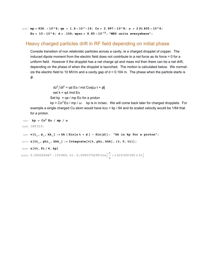
In[16]:= mp = 938. × 10^6; qe = 1.6 × 10^-19; Co = 2.997 × 10^8; ω = 2 Pi 805 × 10^6;

Eo = 10 × 10^6; d = .104; epso = 8.85 × 10-12; "MKS units everywhere";

Heavy charged particles drift in RF field depending on initial phase

Conside transition of non relativistic particles across a cavity, ie a charged dropplet of copper. The induced dipole moment from the electric field does not contribute to a net force as its force = 0 for a uniform field. However it the dropplet has a net charge qd and mass md then there can be a net drift, depending on the phase of when the dropplet is launched. The motion is calculated below. We normal- ize the electric field to 10 MV/m and a cavity gap of d = 0.104 m. The phase when the particle starts is ϕ. dz2dt2 = qd Eo / md Cos[ω t + ϕ] set k = qd /md Eo Set kp = qe / mp Eo for a proton kp = Co2 Eo / mp / ω kp is in m/sec. We will come back later for charged dropplets. For example a single charged Cu atom would have kcu = kp / 64 and its scaled velocity would be 1/64 that for a proton.

In[3]:=

kp = Co2 Eo / mp / ω

Out[3]= 189 319. In[4]:= v[t_, ϕ_, kk_] := kk ( Sin[ω t + ϕ ] - Sin[ϕ]);

"kk is kp for a proton";

In[17]:= z[tt_, phi_, kkk_] := Integrate[v[t, phi, kkk], {t, 0, tt}]; In[18]:= z[tt, Pi / 4, kp] Out[18]= 0.000026467 - 133 869. tt - 0.0000374299 Cos π

4 + 1 610 000 000 π tt

In[5]:= Plot[{v[t, 0, kp], v[t, -Pi / 4, kp]}, {t, 0, 10^-8},

PlotStyle → {Red, Blue}, GridLines → {None, {kp Sin[π / 4]}}, Frame → True, FrameLabel → {"RF cycle time", "velocity", "Proton drift in 10 MV/m RF field\nRed ϕ = 0. Blue ϕ = -π/4\nAverage drift velocity = kp Sin[ϕ", ""}]

Out[5]=

• 2. × 10-9
• 4. × 10-9
• 6. × 10-9
• 8. × 10-9
• 1. × 10-8
• 200000
• 100000

100000 200000 300000 RF cycle time velocity Proton drift in 10 MV/m RF field Red ϕ = 0. Blue ϕ = -π/4 Average drift velocity = kp Sin[ϕ

In[19]:= Plot[{z[tt, 0, kp], z[tt, -Pi / 4, kp]}, {tt, 0, 10^-8},

PlotStyle → {Red, Blue}, GridLines → {None, {kp Sin[π / 4]}}, Frame → True, FrameLabel → {"RF cycle time", "velocity", "Proton drift in 10 MV/m RF field\nRed ϕ = 0. Blue ϕ = -π/4\nAverage drift velocity = kp Sin[ϕ", ""}]

Out[19]=

• 2. × 10-9
• 4. × 10-9
• 6. × 10-9
• 8. × 10-9
• 1. × 10-8

0.0000 0.0002 0.0004 0.0006 0.0008 0.0010 0.0012 0.0014 RF cycle time velocity Proton drift in 10 MV/m RF field Red ϕ = 0. Blue ϕ = -π/4 Average drift velocity = kp Sin[ϕ

From the above we see the average velocity of a proton is k Sin[ϕ] = 189319 Sin[ϕ] meters/sec or 0.23 mm / rf cycle. It would take a proton at max Sin[ϕ] 400 cycles to drift across the cavity. Its peak energy is about 1/2 mp Co^2 β2 . β2 is about 10-6(see above plot). The case for a droplett is modified as its charge/mass ratio will be much smaller for two reasons: the mass is higher by 64 x Number of copper atoms in the droplet and the charge is much smaller than the number of copper atoms.

2 TimeDropletSolidify.nb

Dropplets

Lets consider a dropplet.. Lets estimate the charge possible on a dropplet. A sphere in a uniform field has an induced dipole moment and the max field on its surface is 3 Eo at the pole. he droplet has an induced dipole, the net charge is zero. Suppose we place an additional charge of electrons on the dropplet so that the surface charge is negative everywhere. Since this will be uniform, the net number

• f electrons will be 4 Pi a2 ϵo (3 Eo) / qe. The number of copper atoms is 4/3 Pi a3 /(4/3 Pi 1.25

10^-10)3 where a is the radius of the dropplett and 1.25 10e-10 is the radius of a copper atom in

• meters. So can compute qd / md in terms of the qe / mp by calculating the number of electrons and

number of copper atoms. So the qd / md = 4 Pi a2 ( 3 Eo ϵo /qe) / (a / 1.25 10^-10)3 qe / mp fac[a_] := 4 π a2 ( 3 Eo epso / qe)  a  1.25 × 10-10 3 fac[a] is used to multiply kp (the drift velocity of a proton) and obtain the droplet velocity as a fraction of what the proton drift velocity would be. Note that the surface charge we have used is already very high! and I would expect the charge would be much lower. In any case the above charge means the field at every spot on the droplet is repulsive.

In[6]:= fac[a_] := 4 π a2  3 Eo epso / qe  a  1.25 × 10-10 3 In[7]:= fac[10^-5] kp Out[7]= 0.000771044

Note: a is in meters.. So we see the velocity of drift fpr a 10 μ radius dropplet is 0.7 mm/sec. It takes

• ver 100 sec to cross cavity!

Time constant for sphere to solidify with radiation cooling

In[8]:= Hcu = 209; ρ = 8.9; ϵ = 0.2; σ = 5.67 × 10^-4; Tm = 1358;

Units above mks except length in cm, weight in grms. We calculate how any joules are stored in the latent heat of melting. If the droplet is just starting to solidify, then this heat must be removed before it becomes solid. If the temperature is above 1358 K then it must be first be cooled to this temperature. The cooling is by radiation. The emittance of molten copper is about 0.2. We calculate the cooling in two stages: τc From the initial tenperature Ti to 1358 and then τ the time to get the latent heat of melting out. τ = 1/3 a ρ Hcu / (ϵ σ ( Tm4- 3004)). Above the melting point, the specific heat of copper is constant and equal 0.625 joules/grm up to about 2000 K. So for instance the additional heat from from 1358 to 2000 is about 400 joutes. Integrating, we get τc[a_, Ti_] := - 3 / 5 a ρ .625 Ti-3 - 1358-3  ( ϵ σ)

TimeDropletSolidify.nb 3

The total time to solidify is the sum of these two times. Note: a is in cm! sorry

In[9]:= τ[a_] := 1  3 a ρ Hcu  ϵ σ  Tm4 - 3004 In[10]:= τ[a] Out[10]= 1.61153 × 10-6 a In[11]:= 4  3 Pi a^3 ρ Hcu

"Joules stored in latent heat of fusion times"

Out[11]= 7791.57 Joules stored in latent heat of fusion times a3 In[12]:= 4 Pi a^2 ϵ σ Tm^4 - 300^4 "Joules Radiated/sec

times"

Out[12]= 4.83489 × 109 Joules Radiated/sec

times a2

In[13]:= LogLogPlot[{τ[a 10^-4], τ[a 10^-4] + τc[10^-4 a, 2000]},

{a, 1, 10^3}, PlotStyle → {Red, Blue}, Frame → True, FrameLabel → {"Sphere radius, micron", "t, sec", "Plot of time to solidify\nRed molten state 1358 K->solid\nBlue 2000 K -> solid", ""}]

Out[13]=

1 10 100 1000 10-10 10-9 10-8 10-7 Sphere radius, micron t, sec Plot of time to solidify Red molten state 1358 K->solid Blue 2000 K -> solid

In[14]:= τc[a_, Ti_] := - a ρ .625 Ti-3 - 1358-3  9 ϵ σ In[15]:= τc[1, 1678] Out[15]= 1.02273 × 10-6

Conclusion: Mystery

The cavity has a gap of 0.1 meter. A 100μ drop has a cooling time constant of few times 10-8 sec. To get across the cavity before solidifying its velocity would have to be 107 m/sec!!!! So droplet must come from same side. If so it must be nearby. The splash marks are remarkably symetrical...doesn’t look like a side wise hit. There isn’t molten copper till late in the discharge. How does one eject a charged droplet? I would guess that an expert could estimate haw fast the droplet hit from the splash mark. That would give us

4 TimeDropletSolidify.nb

an estimate of the charge. Notice the little tiny spheres around the splash. I would suggest that they are so small that thier cooling time is <ns and they are solid when they hit.

TimeDropletSolidify.nb 5