h ( x ) } Although we can generally find the best set of weights - - PowerPoint PPT Presentation

1

Class #03: Linear and Polynomial Regression Models

Machine Learning (COMP 135): M. Allen, 27 Jan. 20

1

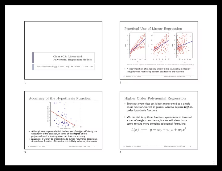
Practical Use of Linear Regression

} A linear model can often radically simplify a data-set, isolating a relatively

straightforward relationship between data-features and outcomes

Monday, 27 Jan. 2020 Machine Learning (COMP 135) 2

50 100 200 300 5 10 15 20 25 TV Sales 10 20 30 40 50 5 10 15 20 25 Radio Sales 20 40 60 80 100 5 10 15 20 25 Newspaper Sales

Ad sales vs. media expenditure (1000’s of units). From: James et al., Intro. to Statistical Learning (Springer, 2017)

2

Accuracy of the Hypothesis Function

} Although we can generally find the best set of weights efficiently, the

exact form of the equation, in terms of the degree of the polynomial used in that equation, can limit our accuracy

} Example: if we try to predict time to tumor recurrence based on a

simple linear function of its radius, this is likely to be very inaccurate

Monday, 27 Jan. 2020 Machine Learning (COMP 135) 3

10 15 20 25 30 10 20 30 40 50 60 70 80 tumor radius (mm?) time to recurrence (months?)

3

Higher Order Polynomial Regression

} Since not every data-set is best represented as a simple

linear function, we will in general want to explore higher-

• rder hypothesis functions

} We can still keep these functions quasi-linear, in terms of

a sum of weights over terms, but we will allow those terms to take more complex polynomial forms, like:

Monday, 27 Jan. 2020 Machine Learning (COMP 135) 4

h(x) ← − y = w0 + w1x + w2x2

4

2 Higher Order Polynomial Regression

} Note: the hypothesis function here is still linear, in terms

• f a sum of coefficients, each multiplied by a single feature

} The same algorithms can find the coefficients that minimize

error, just as before

} What is different, however, are the features themselves

} A feature transformation is a common ML technique } In order to best solve a problem, we generally don’t care what

features we use

} We will often experiment with modifying features to get better

results from existing algorithms

Monday, 27 Jan. 2020 Machine Learning (COMP 135) 5

h(x) ← − y = w0 + w1x + w2x2

5

Higher-Order Regression Solutions

} With an order-2 function, we can fit our data somewhat

better than with the original, order-1 version

Monday, 27 Jan. 2020 Machine Learning (COMP 135) 6

h(x) ← − y = 0.73 + 1.74x + 0.68x2

x y x y

h(x) ← − y = 1.05 + 1.60x

6

Higher-Order Regression Solutions

} It is important to note that the “curves” we get are still linear

}

These are the result of projecting a linear structure in a higher dimensional space back into the dimensions of the original data

Monday, 27 Jan. 2020 Machine Learning (COMP 135) 7

h(x) ← − y = 0.73 + 1.74x + 0.68x2

x y x y

h(x) ← − y = 1.05 + 1.60x

7

Higher-Order Fitting

Order-3 Solution Order-4 Solution

x y x y Monday, 27 Jan. 2020 Machine Learning (COMP 135) 8

8

3 Even Higher-Order Fitting

Order-5 Solution Order-6 Solution

Monday, 27 Jan. 2020 Machine Learning (COMP 135) 9

Order-7 Solution Order-8 Solution

x y x y x y x y

9

The Risk of Overfitting

} An order-9 solution hits all

the data points exactly, but is very “wild” at points that are not given in the data, with high variance

} This is a general problem for

learning: if we over-train, we can end up with a function that is very precise on the data we already have, but will not predict accurately when used on new examples

Monday, 27 Jan. 2020 Machine Learning (COMP 135) 10 x y

10

Defining Overfitting

} T

• precisely understand overfitting, we distinguish between two

types of error:

1.

T rue error: the actual error between the hypothesis and the true function that we want to learn

2.

T raining error: the error observed on our training set of examples, during the learning process

} Overfitting is when: 1.

We have a choice between hypotheses, h1 & h2

2.

We choose h1 because it has lowest training error

3.

Choosing h2 would actually be better, since it will have lowest true error, even if training error is worse

} In general we do not know true error (would essentially need to

already know function we are trying to learn)

} How then can we estimate the true error?

Monday, 27 Jan. 2020 Machine Learning (COMP 135) 11

11

This Week

} Linear and polynomial regression; gradient descent and

gradient ascent; over-fitting and cross validation

} Readings:

} Book sections on linear methods and regression (see class schedule)

} Assignment 01: posted to class Piazza

} Due via Gradescope, 9:00 AM, Wednesday, 29 January

} Office Hours: 237 Halligan

} Mondays, 10:30 AM – Noon } Tuesdays, 9:00 AM – 10:30 AM } TA hours/locations can be found on class site

Monday, 27 Jan. 2020 Machine Learning (COMP 135) 12

12