SLIDE 1
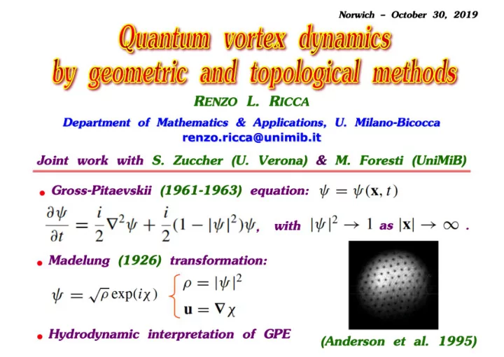
SLIDE 2 Helicity and linking numbers
Helicity H :
H(L n) = u⋅ω
V (ω )
∫
d3X = LkijΓiΓj
i≠j
∑
+ LkiΓ2
i i
∑
where with in .
3
ω = ∇×u ∇⋅u = 0
. .
= 0
,
HGPE
ˆ t
ˆ n
ˆ b
Γ
Under GPE (Salman 2017; Kedia et al. 2018): Theorem (Moffatt 1969; Moffatt & Ricca 1992). Let be a
disjoint union of n vortex tubes in an ideal fluid. (Salman 2017)
SLIDE 3
t = 30 t = 37 t = 51 t = 41.5
Cascade process of Hopf link ( )
SLIDE 4
Reconnection process of iso-phase surface close-up view anti-parallel approach
i) ii)
SLIDE 5
Reconnection process of iso-phase surface anti-parallel reconnection separation
iv) iii)
SLIDE 6
Twist analysis by isophase ribbon construction ribbon construction
SLIDE 7 Writhe and twist contributions (Zuccher & Ricca PRE 2017)
Wr
tot = Wr 1 +Wr 2 + 2Lk12
SLIDE 8 Individual writhe and twist contributions
Writhe remains conserved
across anti-parallel reconnection: (Laing et al. 2015)
Twist remains conserved
across anti-parallel reconnection:
Total writhe and twist decrease
monotonically during the process.
. .
SLIDE 9
where
.
+1 +1 +2 and denotes the standard area of . The weighted area is given by Consider the Pi component of P along the i-direction ( ), and the area of the projected graph along i. Consider the linear momentum (per unit density): where is the area projected along bounded by . Interpretation of momentum in terms of weighted area
SLIDE 10 Theorem (Ricca, 2008; 2012). The linear and angular
momentum P and M of a vortex link of circulation Γ can be expressed in terms of weighted areas of the projected graph regions by , , Linear and angular momentum by weighted area information where , and ( ) denotes the weighted area of the projected graph along the i-direction.
- Corollary. The components of linear and
angular momentum of a vortex tangle can be computed in terms of weighted areas of the projected graph regions of the tangle.
SLIDE 11
Weighted area computation: t = 35 (Zuccher & Ricca PRE 2019)
SLIDE 12
Weighted area computation: t = 37 (Zuccher & Ricca PRE 2019)
SLIDE 13 Resultant momentum of Hopf link and reconnecting rings
10 20 30 40 50 60 70 195 200 205 210 215 t px 10 20 30 40 50 60 70 195 200 205 210 215 t pz 10 20 30 40 50 60 70
2 4 6 8 t py
Pz Py Px P P P P t t Hopf link reconnecting rings t
SLIDE 14 Production of Hopf link and trefoil knot from unlinked loops (Zuccher & Ricca 2019, to be submitted) Hopf link Trefoil knot see movie
time time
P P P P
SLIDE 15 superposition of phase twist Tw = 1 on vortex ring induction of phase twist Tw = 1 on vortex ring
Case B: twist superposition Case A: twist induction
t = 0 t = 0 Physical effects of phase twist (Zuccher & Ricca FDR 2018) phase contour in the
(y-z) plane
SLIDE 16 Biot-Savart induction law:
Case A: twist induction induction of phase twist Tw = 1 on vortex ring
|uξ| U
t = 0
SLIDE 17 Proof. (i) If and are linked Tw1 + Tw2 = 2 : since Γ1 = Γ2 = 1 , H = 0 Lktot = 0
0 = 2Lk12 + (Wr1 + Tw1) + (Wr2 + Tw2) Wr1 = 0 , Wr2 = 0 ; 0 = 2Lk12 + Tw1 + Tw2 Tw1 + Tw2 = 2
We can prove that the lowest energy twist state is given by
L2
+ +
. .
|Tw1| = 1 |Tw2| = 1 Lk12 = +1
L1
Case B: twist superposition
Theorem (Foresti & Ricca 2019). Let be a vortex ring of
Γ1 = 1. A rectilinear, central vortex of Γ2 = 1 can co-exists
if and only if and are linked so that Tw1 + Tw2 = 2 .
L1 L2 L1 L2
SLIDE 18
- Twist. The twist Tw of a unit vector on a curve is defined
by
Zero-twist condition. The unit vector
does not rotate along if and only if it is Fermi-Walker (FW)-transported along , i.e.
L L
.
= 0
∀s ∈ L
, .
Phase-twist. Let
be the ribbon unit vector on the isophase cst.:
.
;
L
(ii) If there is Tw1 such that and are linked: suppose we have only and for simplicity .
L1
L2
L1 = L
Tw1 = Tw = 1
SLIDE 19 ψ = ψ0 + ψ1 + . . . ψ0
, . ,
- Tw ≠ 0 : dispersion relation in presence of winding
; after linearinzing we obtain ,
∇ν ∝ k
(Foresti & Ricca, PRE 2019)
Tw = 0 : dispersion relation for Kelvin waves
Twist injection by phase perturbation with a new dispersion relation given by: