Greedy Algorithms - Gordon Gecko (Michael Douglas) Optimization - - PDF document

1 Analysis of Algorithms

Piyush Kumar

(Lecture e 4: Greedy y Algorithms)

Welcome to 4531 Source: K. Wayne, …

Greed is good. Greed is right. Greed works. Greed clarifies, cuts through, and captures the essence of the evolutionary spirit.

• Gordon Gecko (Michael Douglas)

Greedy Algorithms

• Optimization problem: Min/Max an objective.

– Minimize the total length of a spanning tree. – Minimize the size of a file using compression – … (The mother of all problems)

• Greedy Algorithm

– Attempt to do best at each step without consideration of future consideration

• For some problems, Locally optimal choice leads to global opt.
• Follows “Greed is good” philosophy
• Requires “Optimal Substructure”
• What examples have we already seen?

Greedy Algorithms

• For some problems, “Greed is good” works.
• For some, it finds a good solution which is not global opt

– Heuristics – Approximation Algorithms

• For some, it can do very bad.

Problem of Change

• Vending machine has quarters, nickels, pennies and dimes.

Needs to return N cents change.

• Wanted: An algorithm to return the N cents in minimum

number of coins.

• What do we do?

5

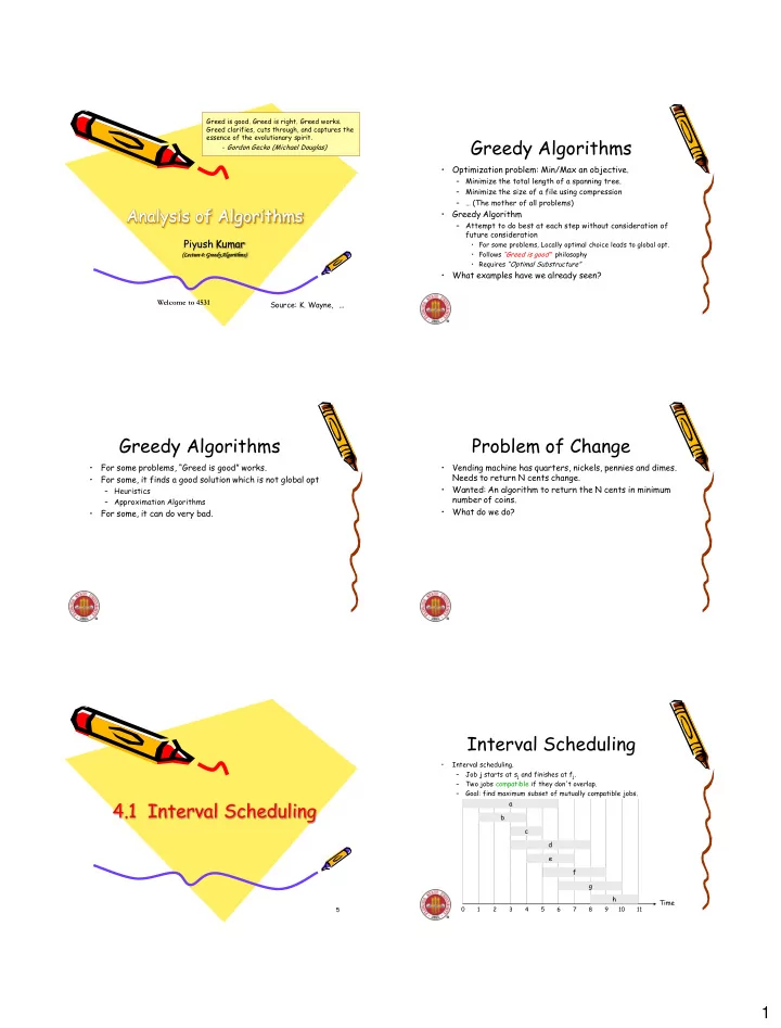
4.1 Interval Scheduling Interval Scheduling

• Interval scheduling.

– Job j starts at sj and finishes at fj. – Two jobs compatible if they don't overlap. – Goal: find maximum subset of mutually compatible jobs. Time

1 2 3 4 5 6 7 8 9 10 11

f g h e a b c d

2

Interval Scheduling: Greedy Algorithms

• Greedy template. Consider jobs in some order. Take each job provided it's

compatible with the ones already taken. – [Earliest start time] Consider jobs in ascending order of start time sj. – [Earliest finish time] Consider jobs in ascending order of finish time fj. – [Shortest interval] Consider jobs in ascending order of interval length fj - sj. – [Fewest conflicts] For each job, count the number of conflicting jobs

• cj. Schedule in ascending order of conflicts cj.

Interval Scheduling: Greedy Algorithms

• Greedy template. Consider jobs in some order. Take each job provided it's

compatible with the ones already taken.

breaks earliest start time breaks shortest interval breaks fewest conflicts

• Greedy algorithm. Consider jobs in increasing order of finish time. Take

each job provided it's compatible with the ones already taken.

• Implementation. O(n log n).

– Remember job j* that was added last to A. – Job j is compatible with A if sj  fj*. Sort jobs by finish times so that f1  f2  ...  fn. A   for j = 1 to n { if (job j compatible with A) A  A  {j} } return A

jobs selected

Interval Scheduling: Greedy Algorithm

Interval Scheduling: Analysis

• Theorem. Greedy algorithm is optimal.
• Pf. (by contradiction)

– Assume greedy is not optimal, and let's see what happens. – Let i1, i2, ... ik denote set of jobs selected by greedy. – Let j1, j2, ... jm denote set of jobs in the optimal solution with i1 = j1, i2 = j2, ..., ir = jr for the largest possible value of r.

j1 j2 jr i1 i1 ir ir+1

. . . Greedy: OPT: jr+1

why not replace job jr+1 with job ir+1? job ir+1 finishes before jr+1

j1 j2 jr i1 i1 ir ir+1

Interval Scheduling: Analysis

• Theorem. Greedy algorithm is optimal.
• Pf. (by contradiction)

– Assume greedy is not optimal, and let's see what happens. – Let i1, i2, ... ik denote set of jobs selected by greedy. – Let j1, j2, ... jm denote set of jobs in the optimal solution with i1 = j1, i2 = j2, ..., ir = jr for the largest possible value of r. . . . Greedy: OPT:

solution still feasible and optimal, but contradicts maximality of r.

ir+1

job ir+1 finishes before jr+1

12

4.1 Interval Partitioning

3

Interval Partitioning

• Interval partitioning.

– Lecture j starts at sj and finishes at fj. – Goal: find minimum number of classrooms to schedule all lectures so that no two occur at the same time in the same room.

• Ex: This schedule uses 4 classrooms to schedule 10 lectures.

Time

9 9:30 10 10:30 11 11:30 12 12:30 1 1:30 2 2:30

h c b a e d g f i j

3 3:30 4 4:30

Interval Partitioning

• Interval partitioning.

– Lecture j starts at sj and finishes at fj. – Goal: find minimum number of classrooms to schedule all lectures so that no two occur at the same time in the same room.

• Ex: This schedule uses only 3.

Time

9 9:30 10 10:30 11 11:30 12 12:30 1 1:30 2 2:30

h c a e f g i j

3 3:30 4 4:30

d b

Interval Partitioning: Lower Bound

• n Optimal Solution
• Def. The depth of a set of open intervals is the maximum number

that contain any given time.

• Key observation. Number of classrooms needed  depth.
• Ex: Depth of schedule below = 3  schedule below is optimal.
• Q. Does there always exist a schedule equal to depth of intervals?

Time

9 9:30 10 10:30 11 11:30 12 12:30 1 1:30 2 2:30

h c a e f g i j

3 3:30 4 4:30

d b

a, b, c all contain 9:30

Interval Partitioning: Greedy Algorithm

• Greedy algorithm. Consider lectures in increasing order of start time:

assign lecture to any compatible classroom.

• Implementation. O(n log n).

– For each classroom k, maintain the finish time of the last job added. – Keep the classrooms in a priority queue. Sort intervals by starting time so that s1  s2  ...  sn. d  0 for j = 1 to n { if (lecture j is compatible with some classroom k) schedule lecture j in classroom k else allocate a new classroom d + 1 schedule lecture j in classroom d + 1 d  d + 1 }

number of allocated classrooms

Interval Partitioning: Greedy Analysis

• Observation. Greedy algorithm never schedules two incompatible lectures in

the same classroom.

• Theorem. Greedy algorithm is optimal.
• Pf.

– Let d = number of classrooms that the greedy algorithm allocates. – Classroom d is opened because we needed to schedule a job, say j, that is incompatible with all d-1 other classrooms. – Since we sorted by start time, all these incompatibilities are caused by lectures that start no later than sj. – Thus, we have d lectures overlapping at time sj + . – Key observation  all schedules use  d classrooms. ▪

18

4.2 Scheduling to Minimize Lateness

4

Scheduling to Minimizing Lateness

• Minimizing lateness problem.

– Single resource processes one job at a time. – Job j requires tj units of processing time and is due at time dj. – If j starts at time sj, it finishes at time fj = sj + tj. – Lateness: j = max { 0, fj - dj }. – Goal: schedule all jobs to minimize maximum lateness L = max j.

• Ex:

1 2 3 4 5 6 7 8 9 10 11 12 13 14 15

d5 = 14 d2 = 8 d6 = 15 d1 = 6 d4 = 9 d3 = 9

lateness = 0 lateness = 2

dj 6 tj 3 1 8 2 2 9 1 3 9 4 4 14 3 5 15 2 6

max lateness = 6

Minimizing Lateness: Greedy Algorithms

• Greedy template. Consider jobs in some order.

– [Shortest processing time first] Consider jobs in ascending

• rder of processing time tj.

– [Earliest deadline first] Consider jobs in ascending order of deadline dj. – [Smallest slack] Consider jobs in ascending order of slack dj - tj.

• Greedy template. Consider jobs in some order.

– [Shortest processing time first] Consider jobs in ascending

• rder of processing time tj.

– [Smallest slack] Consider jobs in ascending order of slack dj - tj.

counterexample counterexample dj tj 100 1 1 10 10 2 dj tj 2 1 1 10 10 2

Minimizing Lateness: Greedy Algorithms

1 2 3 4 5 6 7 8 9 10 11 12 13 14 15

d5 = 14 d2 = 8 d6 = 15 d1 = 6 d4 = 9 d3 = 9

max lateness = 1

Sort n jobs by deadline so that d1  d2  …  dn t  0 for j = 1 to n Assign job j to interval [t, t + tj] sj  t, fj  t + tj t  t + tj

• utput intervals [sj, fj]

Minimizing Lateness: Greedy Algorithm

• Greedy algorithm. Earliest deadline first.

Minimizing Lateness: No Idle Time

• Observation. There exists an optimal schedule with no idle time.
• Observation. The greedy schedule has no idle time.

1 2 3 4 5 6

d = 4 d = 6

7 8 9 10 11

d = 12

1 2 3 4 5 6

d = 4 d = 6

7 8 9 10 11

d = 12

Minimizing Lateness: Inversions

• Def. An inversion in schedule S is a pair of jobs i and j such that:

i < j but j scheduled before i.

• Observation. Greedy schedule has no inversions.
• Observation. If a schedule (with no idle time) has an inversion, it

has one with a pair of inverted jobs scheduled consecutively.

i j

before swap

inversion

5

Minimizing Lateness: Inversions

• Def. An inversion in schedule S is a pair of jobs i and j such that:

i < j but j scheduled before i.

• Claim. Swapping two adjacent, inverted jobs reduces the number of

inversions by one and does not increase the max lateness.

• Pf. Let  be the lateness before the swap, and let  ' be it afterwards.

– 'k = k for all k  i, j – 'i  i – If job j is late: i j i j

before swap after swap

n) (definitio ) ( ) time at finishes ( n) (definitio

i i i i j i j j j

j i d f f j d f d f            

f'j fi inversion

Minimizing Lateness: Analysis of Greedy Algorithm

• Theorem. Greedy schedule S is optimal.
• Pf. Define S* to be an optimal schedule that has

the fewest number of inversions, and let's see what happens. – Can assume S* has no idle time. – If S* has no inversions, then S = S*. – If S* has an inversion, let i-j be an adjacent inversion.

• swapping i and j does not increase the

maximum lateness and strictly decreases the number of inversions

• this contradicts definition of S* ▪

Greedy Analysis Strategies

• Greedy algorithm stays ahead. Show that after each step of the

greedy algorithm, its solution is at least as good as any other algorithm's.

• Exchange argument. Gradually transform any solution to the one

found by the greedy algorithm without hurting its quality.

• Structural. Discover a simple "structural" bound asserting that

every possible solution must have a certain value. Then show that your algorithm always achieves this bound.

28

4.3 Optimal Caching Optimal Offline Caching

• Caching.

– Cache with capacity to store k items. – Sequence of m item requests d1, d2, …, dm. – Cache hit: item already in cache when requested. – Cache miss: item not already in cache when requested: must bring requested item into cache, and evict some existing item, if full.

• Goal. Eviction schedule that minimizes number of

cache misses.

• Ex: k = 2, initial cache = ab,

requests: a, b, c, b, c, a, a, b.

• Optimal eviction schedule: 2 cache misses.

a b a b c b c b c b a b a b c b c a a b a a b b cache requests

Optimal Offline Caching: Farthest-In-Future

• Farthest-in-future. Evict item in the cache that is not requested until

farthest in the future.

• Theorem. [Bellady, 1960s] FF is optimal eviction schedule.
• Pf. Algorithm and theorem are intuitive; proof is subtle.

a b

g a b c e d a b b a c d e a f a d e f g h ...

current cache: c d e f future queries:

cache miss eject this one

6

Reduced Eviction Schedules

• Def. A reduced schedule is a schedule that only inserts an item

into the cache in a step in which that item is requested.

• Intuition. Can transform an unreduced schedule into a reduced
• ne with no more cache misses.

a x an unreduced schedule c a d c a d b a c b a x b a c b a b c a b c a c d a b c a a a b a reduced schedule c a b c a d c a d c a d b a c b a c b a c b a c d a b c a a a b c a a b c a

Reduced Eviction Schedules

• Claim. Given any unreduced schedule S, can transform it into a reduced

schedule S' with no more cache misses.

• Pf. (by induction on number of unreduced items)

– Suppose S brings d into the cache at time t, without a request. – Let c be the item S evicts when it brings d into the cache. – Case 1: d evicted at time t', before next request for d. – Case 2: d requested at time t' before d is evicted. ▪

t t' d c t t' c

S'

d

S

d requested at time t'

t t' d c t t' c

S'

e

S

d evicted at time t', before next request

e

doesn't enter cache at requested time

Case 1 Case 2

Farthest-In-Future: Analysis

• Theorem. FF is optimal eviction algorithm.
• Pf. (by induction on number or requests j)
• Let S be reduced schedule that satisfies invariant through j
• requests. We produce S' that satisfies invariant after j+1

requests. – Consider (j+1)st request d = dj+1. – Since S and SFF have agreed up until now, they have the same cache contents before request j+1. – Case 1: (d is already in the cache). S' = S satisfies invariant. – Case 2: (d is not in the cache and S and SFF evict the same element). S' = S satisfies invariant.

Invariant: There exists an optimal reduced schedule S that makes the same eviction schedule as SFF through the first j+1 requests. j

Farthest-In-Future: Analysis

• Pf. (continued)

– Case 3: (d is not in the cache; SFF evicts e; S evicts f  e).

• begin construction of S' from S by evicting e instead of f
• now S' agrees with SFF on first j+1 requests; we show that having

element f in cache is no worse than having element e same f same f e e S S' j same d same f d e S S' j+1

Farthest-In-Future: Analysis

• Let j' be the first time after j+1 that S and S' take a different action, and

let g be item requested at time j'. – Case 3a: g = e. Can't happen with Farthest-In-Future since there must be a request for f before e. – Case 3b: g = f. Element f can't be in cache of S, so let e' be the element that S evicts.

• if e' = e, S' accesses f from cache; now S and S' have same cache
• if e'  e, S' evicts e' and brings e into the cache; now S and S'

have the same cache

same

e

same

f S S' j'

Note: S' is no longer reduced, but can be transformed into a reduced schedule that agrees with SFF through step j+1 must involve e or f (or both)

Farthest-In-Future: Analysis

• Let j' be the first time after j+1 that S and S' take a different action, and

let g be item requested at time j'. – Case 3c: g  e, f. S must evict e. Make S' evict f; now S and S' have the same cache. ▪

same

g

same

g S S' j'

• therwise S' would take the same action

same

e

same

f S S' j'

must involve e or f (or both)

7

Caching Perspective

• Online vs. offline algorithms.

– Offline: full sequence of requests is known a priori. – Online (reality): requests are not known in advance. – Caching is among most fundamental online problems in CS.

• LIFO. Evict page brought in most recently.
• LRU. Evict page whose most recent access was earliest.
• Theorem. FF is optimal offline eviction algorithm.

– Provides basis for understanding and analyzing online algorithms. – LRU is k-competitive. [Section 13.8] – LIFO is arbitrarily bad.

FF with direction of time reversed!