Greedy algorithms: greed is good? Greedy algorithms Shortest paths - - PowerPoint PPT Presentation

Greedy algorithms

Shortest paths in weighted graphs Tyler Moore

CSE 3353, SMU, Dallas, TX

Lecture 13

Some slides created by or adapted from Dr. Kevin Wayne. For more information see http://www.cs.princeton.edu/~wayne/kleinberg-tardos. Some code reused from Python Algorithms by Magnus Lie Hetland.

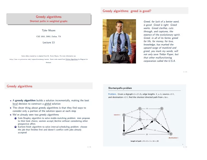
Greedy algorithms: greed is good?

Greed, for lack of a better word, is good. Greed is right. Greed

• works. Greed clarifies, cuts

through, and captures, the essence of the evolutionary spirit. Greed, in all of its forms; greed for life, for money, for love, knowledge, has marked the upward surge of mankind and greed, you mark my words, will not only save Teldar Paper, but that other malfunctioning corporation called the U.S.A.

2 / 24

Greedy algorithms

A greedy algorithm builds a solution incrementally, making the best local decision to construct a global solution The clever thing about greedy algorithms is that they find ways to consider only a portion of the solution space at each step We’ve already seen two greedy algorithms

1

Gale-Shapley algorithm to solve stable-matching problem: men propose to their best choice, women accept/decline without considering other prospective offers

2

Earliest-finish algorithm to solve interval-scheduling problem: choose the job that finishes first and doesn’t conflict with jobs already accepted

3 / 24

• Problem. Given a digraph , edge lengths

≥, source ∈,

and destination ∈, find the shortest directed path from to .

• 3

7 1 3

• 6

8 5 7 5 4 15 3 12 20 13 9

• 4

5 2 6 9 4 1 11 4 / 24

• 4

5 / 24

PERT/CPM. Map routing. Seam carving. Robot navigation. Texture mapping. Typesetting in LaTeX. Urban traffic planning. Telemarketer operator scheduling. Routing of telecommunications messages. Network routing protocols (OSPF

, BGP , RIP).

Optimal truck routing through given traffic congestion pattern.

5

• 6 / 24

The many cases of finding shortest paths

We’ve already seen how to calculate the shortest path in an unweighted graph (BFS traversal) We’ll now study how to compute the shortest path in different circumstances for weighted graphs

1

Single-source shortest path on a weighted DAG

2

Single-source shortest path on a weighted graph with nonnegative weights (Dijkstra’s algorithm)

3

Single-source shortest path on a weighted graph including negative weights (Bellman-Ford algorithm)

7 / 24

Weighted Graph Data Structures

a b d c e f h g

2 1 3 9 4 4 3 8 7 5 2 2 2 1 6 9 8

Nested Adjacency Dictionaries w/ Edge Weights

N = { ’ a ’ : { ’ b ’ : 2 , ’ c ’ : 1 , ’ d ’ : 3 , ’ e ’ : 9 , ’ f ’ :4 } , ’ b ’ :{ ’ c ’ : 4 , ’ e ’ :3 } , ’ c ’ : { ’ d ’ : 8} , ’ d ’ :{ ’ e ’ : 7 } , ’ e ’ : { ’ f ’ : 5} , ’ f ’ : { ’ c ’ : 2 , ’ g ’ : 2 , ’ h ’ : 2 } , ’ g ’ : { ’ f ’ : 1 , ’ h ’ :6 } , ’ h ’ :{ ’ f ’ : 9 , ’ g ’ :8} } > > > ’ b ’ i n N[ ’ a ’ ] # Neighborhood membership True > > > l e n (N[ ’ f ’ ] ) # Degree 3 > > > N[ ’ a ’ ] [ ’ b ’ ] # Edge weight f o r ( a , b ) 2

8 / 24

Shortest paths in DAGs

Recursive approach to finding the shortest path from a to z

1

Assume we already know the distance d(v) to z for each of a’s neighbors v ∈ G[a]

2

Select the neighbor v that minimizes d(v) + W (a, v)

9 / 24

Recursive solution to finding shortest path in DAGs

def r e c d a g s p (W, s , t ) : #Shortest path from s to t @memo #Memoize f def d(u ) : #Distance from u to t i f u == t : return 0# We ’ re the re ! # Return the best

• f

every f i r s t step return min (W[ u ] [ v]+d( v ) for v in W[ u ] ) return d( s ) #Apply f to a c t u a l s t a r t node

10 / 24

Shortest paths in DAGs: Iterative approach

The iterative solution is a bit more complicated

1

We must start with a topological sort

2

Keep track of an upper bound on the distance from a to each node, initialized to ∞

3

Go through each vertex and relax the distance estimate by inspecting the path from the vertex to its neighbor

In general, relaxing an edge (u, v) consists of testing whether we can shorten the path to v found so far by going through u; if we can, we update d[v] with the new value Running time: Θ(m + n)

11 / 24

Relaxing edges

s v u

1: d[v] = 13 2 : W [ u ] [ v ] = 3 2: d[u] = 7

12 / 24

Relaxing edges

s v u

2 : W [ u ] [ v ] = 3 2: d[u] = 7 3: d[v] = 13 10 i n f = f l o a t ( ’ i n f ’ ) def r e l a x (W, u , v , D, P ) : d = D. get (u , i n f ) + W[ u ] [ v ]# P o s s i b l e s h o r t c u t estimate i f d < D. get ( v , i n f ) : # I s i t r e a l l y a s h o r t c u t ? D[ v ] , P[ v ] = d , u # Update estimate and parent return True # There was a change !

12 / 24

Iterative solution to finding shortest path in DAGs

def dag sp (W, s , t ) : #Shorte st path from s to t d = {u : f l o a t ( ’ i n f ’ ) for u in W} # Distance e s t i m a t e s d [ s ] = 0 #S ta rt node : Zero d i s t a n c e for u in t o p s o r t (W) : #In top−s o r t e d

• rder . . .

i f u == t : break #Have we a r r i v e d ? for v in W[ u ] : #For each out−edge . . . d [ v ] = min (d [ v ] , d [ u ] + W[ u ] [ v ] ) # Relax the edge return d [ t ] #Distance to t ( from s )

13 / 24

Shortest-paths on weighted DAG example

a b c e d

1 5 6 7 3 3 5 1

a b c e d Topological sort: a, c, b, d, e d[Node]: upper bd. dist. from a Node init. 1 (u=a) 2 (u=c) 3 (u=b) 4 (u=d) 5 (u=e) a b ∞ 15 13 13 13 13 c ∞ 6 6 6 6 6 d ∞ ∞ 9 9 9 9 e ∞ ∞ 11 11 10 10

14 / 24

Shortest-paths on weighted DAG: exercise

15 / 24

But what if there are cycles?

With a DAG, we can select the order in which to visit nodes based on the topological sort With cycles we can’t easily determine the best order If there are no negative edges, we can traverse from the starting vertex, visiting nodes in order of their estimated distance from the starting vertex In Dijkstra’s algorithm, we use a priority queue based on minimum estimated distance from the source to select which vertices to visit Running time: Θ((m + n) lg n) Dijkstra’s algorithm combines approaches seen in other algorithms

1

Node discovery: bit like breadth-first traversal

2

Node visitation: selected using priority queue

3

Shortest path calculation: uses relaxation as in algorithm for shortest paths in DAGs

16 / 24

Greedy approach. Maintain a set of explored nodes for which algorithm has determined the shortest path distance from to .

Initialize . Repeatedly choose unexplored node which minimizes

6

• s

v u

• shortest path to some node u in explored part,

followed by a single edge (u, v)

• e

18 / 24

Greedy approach. Maintain a set of explored nodes for which algorithm has determined the shortest path distance from to .

Initialize . Repeatedly choose unexplored node which minimizes

add to , and set π.

7

• s

v u

• e
• shortest path to some node u in explored part,

followed by a single edge (u, v)

19 / 24

• Invariant. For each node ∈ is the length of the shortest ↝ path.
• Pf. [ by induction on ]

Base case: is easy since and . Inductive hypothesis: Assume true for ≥.

Let be next node added to , and let be the final edge. The shortest ↝ path plus is an ↝ path of length π. Consider any ↝ path . We show that it is no shorter than π. Let be the first edge in that leaves,

and let be the subpath to .

is already too long as soon as it reaches .

• s

8

• ≥
• nonnegative

lengths

v u y P P' x

Dijkstra chose v instead of y

≥π

definition

• f π(y)

≥π

inductive hypothesis

≥

• ▪

20 / 24

9

• Critical optimization 1. For each unexplored node , explicitly

maintain π instead of computing directly from formula:

For each ∉π can only decrease (because only increases). More specifically, suppose is added to and there is an edge

leaving . Then, it suffices to update: Critical optimization 2. Use a priority queue to choose the unexplored node that minimizes π.

• π
• ∈ 

ππ

• 21 / 24

Dijkstra’s algorithm

from heapq import heappush , heappop def d i j k s t r a (G, s ) : D, P, Q, S = { s :0} , {} , [ ( 0 , s ) ] , s e t () # Est . , tree , queue , v i s while Q: # S t i l l unprocessed nodes ? , u = heappop (Q) # Node with lowest estimate i f u in S : continue # Already v i s i t e d ? Skip i t S . add (u) # We ’ ve v i s i t e d i t now for v in G[ u ] : # Go through a l l i t s neighbors r e l a x (G, u , v , D, P) # Relax the

• ut−edge

heappush (Q, (D[ v ] , v ))# Add to queue , w/ e s t . as p r i return D, P # F i n a l D and P returned

22 / 24

Dijkstra’s algorithm example

a b c e d

1 5 1 2 9 2 3 4 6 7

a b c e d d[Node]: upper bd. dist. from a Node init. 1 (u=a) 2 (u=c) 3 (u=e) 4 (u=b) 5 (u=d) a b ∞ 10 8 8 8 8 c ∞ 5 5 5 5 5 d ∞ ∞ 14 13 9 9 e ∞ ∞ 7 7 7 7

23 / 24

Dijkstra’s algorithm: exercise

24 / 24