
SLIDE 1
✬ ✫ ✩ ✪
Graphs
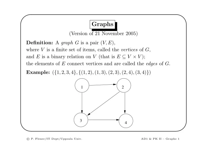
(Version of 21 November 2005) Definition: A graph G is a pair (V, E), where V is a finite set of items, called the vertices of G, and E is a binary relation on V (that is E ⊆ V × V ); the elements of E connect vertices and are called the edges of G. Example: ({1, 2, 3, 4}, {(1, 2), (1, 3), (2, 3), (2, 4), (3, 4)})
1 2 3 4
c
- P. Flener/IT Dept/Uppsala Univ.
AD1 & PK II – Graphs 1