
SLIDE 1
Graphs 1
Graphs
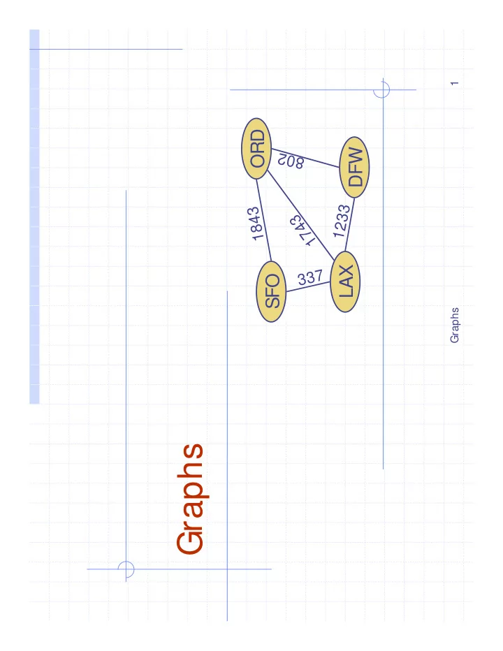
ORD DFW SFO LAX
802 1 7 4 3 1843 1233 337
Graphs Outline and Reading Graphs (12.1) Definition Applications - - PDF document
1 ORD DFW 802 1233 1843 3 4 7 1 LAX 337 SFO Graphs Graphs Outline and Reading Graphs (12.1) Definition Applications Terminology Properties ADT Data structures for graphs (12.2) Edge list structure
Graphs 1
802 1 7 4 3 1843 1233 337
Graphs 2
Definition Applications Terminology Properties ADT
Edge list structure Adjacency list structure Adjacency matrix structure
Graphs 3
A graph is a pair (V, E), where
V is a set of nodes, called vertices E is a collection of pairs of vertices, called edges
Example:
mileage of the route
8 4 9 802 1 3 8 7 1 7 4 3 1843 1099 1120 1233 337 2555 142
Graphs 4
Directed edge
Undirected edge
Directed graph
Undirected graph
Graphs 5
John David Paul
brown.edu cox.net
cs.brown.edu
att.net qwest.net
math.brown.edu cslab1b cslab1a
Printed circuit board Integrated circuit
Highway network Flight network
Local area network Internet Web
Entity-relationship diagram
Graphs 6
End vertices (or endpoints) of an edge
Edges incident on a vertex
Adjacent vertices
Degree of a vertex
Parallel edges
Self-loop
Graphs 7
Path
vertices and edges
followed by its endpoints
Simple path
and edges are distinct
Examples
path that is not simple
Graphs 8
Cycle
vertices and edges
followed by its endpoints
Simple cycle
and edges are distinct
Examples
simple cycle
is a cycle that is not simple
Graphs 9
n
number of vertices
m
number of edges
deg(v)
degree of vertex v
Proof: each edge is counted twice
In an undirected graph with no self-loops and no multiple edges
m ≤ n (n − 1)/2
Proof: each vertex has degree at most (n − 1)
n = 4 m = 6 deg(v) = 3
Graphs 10
Vertices and edges
Accessor methods
Update methods
Generic methods
Graphs 11
Vertex object
vertex sequence
Edge object
edge sequence
Vertex sequence
Edge sequence
v u w a c b a z d u v w z b c d
Graphs 12
Edge list structure Incidence sequence for each vertex
references to edge
edges
Augmented edge
associated positions in incidence sequences of end vertices u v w a b a u v w b
Graphs 13
Edge list structure Augmented vertex
associated with vertex
2D-array adjacency array
vertices
nonadjacent vertices
The “old fashioned” version just has 0 for no edge and 1 for edge
u v w a b 2 1 2 1
∅ ∅ ∅ ∅ ∅
a u v w 1 2 b
Graphs 14
n vertices, m edges
no parallel edges no self-loops Bounds are “big-Oh”
Graphs 15
D B A C E
Graphs 16
Subgraph Connectivity Spanning trees and forests
Algorithm Example Properties Analysis
Path finding Cycle finding
Graphs 17
The vertices of S are a
subset of the vertices of G
The edges of S are a
subset of the edges of G
Subgraph Spanning subgraph
Graphs 18
Connected graph Non connected graph with two connected components
Graphs 19
T is connected T has no cycles
This definition of tree is different from the one of a rooted tree
Tree Forest
Graphs 20
A spanning tree of a connected graph is a spanning subgraph that is a tree A spanning tree is not unique unless the graph is a tree Spanning trees have applications to the design
networks A spanning forest of a graph is a spanning subgraph that is a forest Graph Spanning tree
Graphs 21
Visits all the vertices and
edges of G
Determines whether G is
connected
Computes the connected
components of G
Computes a spanning
forest of G
Find and report a path
between two given vertices
Find a cycle in the graph
Graphs 22
The algorithm uses a mechanism for setting and getting “labels” of vertices and edges
Algorithm DFS(G, v) Input graph G and a start vertex v of G Output labeling of the edges of G in the connected component of v as discovery edges and back edges setLabel(v, VISITED) for all e ∈ G.incidentEdges(v) if getLabel(e) = UNEXPLORED w ← opposite(v,e) if getLabel(w) = UNEXPLORED setLabel(e, DISCOVERY) DFS(G, w) else setLabel(e, BACK) Algorithm DFS(G) Input graph G Output labeling of the edges of G as discovery edges and back edges for all u ∈ G.vertices() setLabel(u, UNEXPLORED) for all e ∈ G.edges() setLabel(e, UNEXPLORED) for all v ∈ G.vertices() if getLabel(v) = UNEXPLORED DFS(G, v)
Graphs 23
D B A C E D B A C E D B A C E
A
A
Graphs 24
D B A C E D B A C E D B A C E D B A C E
Graphs 25
We mark each
intersection, corner and dead end (vertex) visited
We mark each corridor
(edge ) traversed
We keep track of the
path back to the entrance (start vertex) by means of a rope (recursion stack)
Graphs 26
D B A C E
Graphs 27
Recall that Σv deg(v) = 2m
Graphs 28
We can specialize the DFS algorithm to find a path between two given vertices u and z We call DFS(G, u) with u as the start vertex We use a stack S to keep track of the path between the start vertex and the current vertex As soon as destination vertex z is encountered, we return the path as the contents of the stack
Algorithm pathDFS(G, v, z) setLabel(v, VISITED) S.push(v) if v = z return S.elements() for all e ∈ G.incidentEdges(v) if getLabel(e) = UNEXPLORED w ← opposite(v,e) if getLabel(w) = UNEXPLORED setLabel(e, DISCOVERY) S.push(e) pathDFS(G, w, z) S.pop(e) else setLabel(e, BACK) S.pop(v)
Graphs 29
We can specialize the DFS algorithm to find a simple cycle We use a stack S to keep track of the path between the start vertex and the current vertex As soon as a back edge
we return the cycle as the portion of the stack from the top to vertex w
Algorithm cycleDFS(G, v, z) setLabel(v, VISITED) S.push(v) for all e ∈ G.incidentEdges(v) if getLabel(e) = UNEXPLORED w ← opposite(v,e) S.push(e) if getLabel(w) = UNEXPLORED setLabel(e, DISCOVERY) pathDFS(G, w, z) S.pop(e) else T ← new empty stack repeat
T.push(o) until o = w return T.elements() S.pop(v)
Graphs 30
C B A E D
L0 L1
F
L2
Graphs 31
Algorithm Example Properties Analysis Applications
Comparison of applications Comparison of edge labels
Graphs 32
Visits all the vertices and
edges of G
Determines whether G is
connected
Computes the connected
components of G
Computes a spanning
forest of G
Find and report a path
with the minimum number of edges between two given vertices
Find a simple cycle, if
there is one
Graphs 33
The algorithm uses a mechanism for setting and getting “labels” of vertices and edges
Algorithm BFS(G, s) L0 ← new empty sequence L0.insertLast(s) setLabel(s, VISITED) i ← 0 while ¬Li.isEmpty() Li +1 ← new empty sequence for all v ∈ Li.elements() for all e ∈ G.incidentEdges(v) if getLabel(e) = UNEXPLORED w ← opposite(v,e) if getLabel(w) = UNEXPLORED setLabel(e, DISCOVERY) setLabel(w, VISITED) Li +1.insertLast(w) else setLabel(e, CROSS) i ← i +1 Algorithm BFS(G) Input graph G Output labeling of the edges and partition of the vertices of G for all u ∈ G.vertices() setLabel(u, UNEXPLORED) for all e ∈ G.edges() setLabel(e, UNEXPLORED) for all v ∈ G.vertices() if getLabel(v) = UNEXPLORED BFS(G, v)
Graphs 34
C B A E D
A
A
L0 L1
F C B A E D
L0 L1
F C B A E D
L0 L1
F
Graphs 35
C B A E D
L0 L1
F C B A E D
L0 L1
F
L2
C B A E D
L0 L1
F
L2
C B A E D
L0 L1
F
L2
Graphs 36
C B A E D
L0 L1
F
L2
C B A E D
L0 L1
F
L2
C B A E D
L0 L1
F
L2
Graphs 37
Gs: connected component of s
BFS(G, s) visits all the vertices and
edges of Gs
The discovery edges labeled by
BFS(G, s) form a spanning tree Ts
For each vertex v in Li
edges
least i edges C B A E D
L0 L1
F
L2
C B A E D F
Graphs 38
Recall that Σv deg(v) = 2m
Graphs 39
Compute the connected components of G Compute a spanning forest of G Find a simple cycle in G, or report that G is a
Given two vertices of G, find a path in G between
Graphs 40
C B A E D
L0 L1
F
L2
C B A E D F
√
Biconnected components
√
Shortest paths
√ √
Spanning forest, connected components, paths, cycles
Graphs 41
w is an ancestor of v in
the tree of discovery edges
w is in the same level as
v or in the next level in
the tree of discovery edges
C B A E D
L0 L1
F
L2
C B A E D F
Graphs 42
JFK BOS MIA ORD LAX DFW SFO
Graphs 43
Directed DFS Strong connectivity
The Floyd-Warshall Algorithm
Topological Sorting
Graphs 44
Short for “directed graph”
flights task scheduling
Graphs 45
Each edge goes in one direction:
Edge (a,b) goes from a to b, but not b to a.
Graphs 46
The good life ics141 ics131 ics121 ics53 ics52 ics51 ics23 ics22 ics21 ics161 ics151 ics171
Graphs 47
Graphs 48
A C E D A C E B D F
Graphs 49
Graphs 50
If there’s a w not visited, print “no”.
If there’s a w not visited, print “no”. Else, print “yes”.
a d c b e f g a d c b e f g
Graphs 51
Graphs 52
G* has the same vertices
if G has a directed path
Graphs 53
O(n(n+ m))
Graphs 54
Graphs 55
Floyd-Warshall’s algorithm numbers the vertices of G as
v1 , …, vn and computes a
series of digraphs G0, …, Gn
G0=G Gk has a directed edge (vi, vj)
if G has a directed path from
vi to vj with intermediate
vertices in the set {v1 , …, vk}
We have that Gn = G* In phase k, digraph Gk is computed from Gk − 1 Running time: O(n3), assuming areAdjacent is O(1) (e.g., adjacency matrix)
Algorithm FloydWarshall(G) Input digraph G Output transitive closure G* of G i ← 1 for all v ∈ G.vertices() denote v as vi i ← i + 1 G0 ← G for k ← 1 to n do Gk ← Gk − 1 for i ← 1 to n (i ≠ k) do for j ← 1 to n (j ≠ i, k) do if Gk − 1.areAdjacent(vi, vk) ∧ Gk − 1.areAdjacent(vk, vj) if ¬Gk.areAdjacent(vi, vj) Gk.insertDirectedEdge(vi, vj , k) return Gn
Graphs 56
JFK BOS MIA ORD LAX DFW SFO
Graphs 57
JFK BOS MIA ORD LAX DFW SFO
Graphs 58
JFK BOS MIA ORD LAX DFW SFO
Graphs 59
JFK BOS MIA ORD LAX DFW SFO
Graphs 60
JFK BOS MIA ORD LAX DFW SFO
Graphs 61
JFK MIA ORD LAX DFW SFO
BOS
Graphs 62
JFK MIA ORD LAX DFW SFO
BOS
Graphs 63
JFK MIA ORD LAX DFW SFO
BOS
Graphs 64
A directed acyclic graph (DAG) is a digraph that has no directed cycles A topological ordering of a digraph is a numbering
v1 , …, vn
edge (vi , vj), we have i < j Example: in a task scheduling digraph, a topological ordering a task sequence that satisfies the precedence constraints Theorem A digraph admits a topological
Graphs 65
write c.s. program play
wake up eat nap study computer sci. more c.s. work out sleep dream about graphs
A typical day
1 2 3 4 5 6 7 8 9 10 11 Go out w/ friends
Graphs 66
Method TopologicalSort(G) H ← G // Temporary copy of G n ← G.numVertices() while H is not empty do Let v be a vertex with no outgoing edges Label v ← n n ← n - 1 Remove v from H
Graphs 67
Algorithm topologicalDFS(G, v) Input graph G and a start vertex v of G Output labeling of the vertices of G in the connected component of v setLabel(v, VISITED) for all e ∈ G.incidentEdges(v) if getLabel(e) = UNEXPLORED w ← opposite(v,e) if getLabel(w) = UNEXPLORED setLabel(e, DISCOVERY) topologicalDFS(G, w) else {e is a forward or cross edge} Label v with topological number n n ← n - 1 Algorithm topologicalDFS(G) Input dag G Output topological ordering of G n ← G.numVertices() for all u ∈ G.vertices() setLabel(u, UNEXPLORED) for all e ∈ G.edges() setLabel(e, UNEXPLORED) for all v ∈ G.vertices() if getLabel(v) = UNEXPLORED topologicalDFS(G, v)
Graphs 68
Graphs 69
Graphs 70
Graphs 71
Graphs 72
Graphs 73
Graphs 74
Graphs 75
Graphs 76
Graphs 77
Graphs 78
C B A E D F
3 2 8 5 8 4 8 7 1 2 5 2 3 9
Graphs 79
Shortest path problem Shortest path properties
Algorithm Edge relaxation
Graphs 80
In a weighted graph, each edge has an associated numerical value, called the weight of the edge Edge weights may represent distances, costs, etc. Example:
distance in miles between the endpoint airports
8 4 9 802 1 3 8 7 1 7 4 3 1843 1099 1120 1233 337 2555 142 1205
Graphs 81
Given a weighted graph and two vertices u and v, we want to find a path of minimum total weight between u and v.
Example:
Applications
8 4 9 802 1 3 8 7 1 7 4 3 1843 1099 1120 1233 337 2555 142 1205
Graphs 82
Property 1:
A subpath of a shortest path is itself a shortest path
Property 2:
There is a tree of shortest paths from a start vertex to all the other vertices
Example:
Tree of shortest paths from Providence
8 4 9 802 1 3 8 7 1 7 4 3 1843 1099 1120 1233 337 2555 142 1205
Graphs 83
The distance of a vertex
v from a vertex s is the
length of a shortest path between s and v Dijkstra’s algorithm computes the distances
given start vertex s Assumptions:
undirected
nonnegative
We grow a “cloud” of vertices, beginning with s and eventually covering all the vertices We store with each vertex v a label d(v) representing the distance of v from s in the subgraph consisting of the cloud and its adjacent vertices At each step
u outside the cloud with the
smallest distance label, d(u)
vertices adjacent to u (edge
relaxation)
Graphs 84
Consider an edge e = (u,z) such that
u is the vertex most recently
added to the cloud
z is not in the cloud
The relaxation of edge e updates distance d(z) as follows:
d(z) ← min{d(z),d(u) + weight(e)}
d(z) = 75
d(u) = 50 10 z s u
d(z) = 60
d(u) = 50 10 z s u e e
Graphs 85
C B A E D F
4 2 8 ∞ ∞ 4 8 7 1 2 5 2 3 9
C B A E D F
3 2 8 5 11 4 8 7 1 2 5 2 3 9
C B A E D F
3 2 8 5 8 4 8 7 1 2 5 2 3 9
C B A E D F
3 2 7 5 8 4 8 7 1 2 5 2 3 9
Graphs 86
C B A E D F
3 2 7 5 8 4 8 7 1 2 5 2 3 9
C B A E D F
3 2 7 5 8 4 8 7 1 2 5 2 3 9
Graphs 87
A priority queue stores the vertices outside the cloud
Locator-based methods
insert(k,e) returns a
locator
replaceKey(l,k) changes
the key of an item
We store two labels with each vertex:
queue
Algorithm DijkstraDistances(G, s) Q ← new heap-based priority queue for all v ∈ G.vertices() if v = s setDistance(v, 0) else setDistance(v, ∞) l ← Q.insert(getDistance(v), v) setLocator(v,l) while ¬Q.isEmpty() u ← Q.removeMin() for all e ∈ G.incidentEdges(u) { relax edge e } z ← G.opposite(u,e) r ← getDistance(u) + weight(e) if r < getDistance(z) setDistance(z,r) Q.replaceKey(getLocator(z),r)
Graphs 88
Graph operations
Label operations
Priority queue operations
queue, where each insertion or removal takes O(log n) time
times, where each key change takes O(log n) time
Dijkstra’s algorithm runs in O((n + m) log n) time provided the graph is represented by the adjacency list structure
The running time can also be expressed as O(m log n) since the graph is connected
Graphs 89
We can extend Dijkstra’s algorithm to return a tree of shortest paths from the start vertex to all
We store with each vertex a third label:
shortest path tree
In the edge relaxation step, we update the parent label
Algorithm DijkstraShortestPathsTree(G, s) … for all v ∈ G.vertices() … setParent(v, ∅) … for all e ∈ G.incidentEdges(u) { relax edge e } z ← G.opposite(u,e) r ← getDistance(u) + weight(e) if r < getDistance(z) setDistance(z,r) setParent(z,e) Q.replaceKey(getLocator(z),r)
Graphs 90
C B A E D F
3 2 7 5 8 4 8 7 1 2 5 2 3 9
Suppose it didn’t find all shortest
vertex the algorithm processed.
When the previous node, D, on the
true shortest path was considered, its distance was correct.
But the edge (D,F) was relaxed at
that time!
Thus, so long as d(F)> d(D), F’s
distance cannot be wrong. That is, there is no wrong vertex.
Graphs 91
If a node with a negative
incident edge were to be added late to the cloud, it could mess up distances for vertices already in the cloud.
C B A E D F
4 5 7 5 9 4 8 7 1 2 5 6
Graphs 92
Works even with negative- weight edges Must assume directed edges (for otherwise we would have negative- weight cycles) Iteration i finds all shortest paths that use i edges. Running time: O(nm). Can be extended to detect a negative-weight cycle if it exists
Algorithm BellmanFord(G, s) for all v ∈ G.vertices() if v = s setDistance(v, 0) else setDistance(v, ∞) for i ← 1 to n-1 do for each e ∈ G.edges() { relax edge e } u ← G.origin(e) z ← G.opposite(u,e) r ← getDistance(u) + weight(e) if r < getDistance(z) setDistance(z,r)
Graphs 93
∞
∞ ∞ ∞ ∞ ∞ 4 8 7 1
5
3 9 ∞ ∞ ∞ ∞ 4 8 7 1
5 3 9
8 4 ∞ 4 8 7 1
5 3 9 ∞ 8
4
5 6 1 9
5 1
9 4 8 7 1
5
3 9 4
Graphs 94
Works even with negative-weight edges Uses topological order Uses simple data structures Is much faster than Dijkstra’s algorithm Running time: O(n+ m).
Algorithm DagDistances(G, s) for all v ∈ G.vertices() if v = s setDistance(v, 0) else setDistance(v, ∞) Perform a topological sort of the vertices for u ← 1 to n do {in topological order} for each e ∈ G.outEdges(u) { relax edge e } z ← G.opposite(u,e) r ← getDistance(u) + weight(e) if r < getDistance(z) setDistance(z,r)
Graphs 95
∞
∞ ∞ ∞ ∞ ∞ 4 8 7 1
5
3 9 ∞ ∞ ∞ ∞ 4 8 7 1
5 3 9
8 4 ∞ 4 8 7 1
5 3 9 ∞
4
1 7
5 1
7 4 8 7 1
5
3 9 4
1 1 2 4 3 6 5 1 2 4 3 6 5
8
1 2 4 3 6 5 1 2 4 3 6 5
5
(two steps)
Graphs 96
Find the distance between every pair of vertices in a weighted directed graph G. We can make n calls to Dijkstra’s algorithm (if no negative edges), which takes O(nmlog n) time. Likewise, n calls to Bellman-Ford would take O(n2m) time. We can achieve O(n3) time using dynamic programming (similar to the Floyd-Warshall algorithm).
Algorithm AllPair(G) {assumes vertices 1,…,n} for all vertex pairs (i,j) if i = j D0[i,i] ← 0 else if (i,j) is an edge in G D0[i,j] ← weight of edge (i,j) else D0[i,j] ← + ∞ for k ← 1 to n do for i ← 1 to n do for j ← 1 to n do Dk[i,j] ← min{Dk-1[i,j], Dk-1[i,k]+Dk-1[k,j]} return Dn
k j i
Uses only vertices numbered 1,…,k-1 Uses only vertices numbered 1,…,k-1 Uses only vertices numbered 1,…,k (compute weight of this edge)
Graphs 97
JFK BOS MIA ORD LAX DFW SFO BWI PVD 867 2704 187 1258 849 144 740 1391 184 946 1090 1121 2342 1846 621 802 1464 1235 337
Graphs 98
Definitions A crucial fact
Graphs 99
Spanning subgraph
containing all the vertices of G
Spanning tree
itself a (free) tree
Minimum spanning tree (MST)
graph with minimum total edge weight
Applications
10 1 9 8 6 3 2 5 7 4
Graphs 100
Cycle Property:
spanning tree of a weighted graph G
that is not in T and let C be the cycle formed by e with T
weight(f) ≤ weight(e)
Proof:
can get a spanning tree
replacing e with f 8 4 2 3 6 7 7 9 8
e
C
f
8 4 2 3 6 7 7 9 8
C
e f
Replacing f with e yields a better spanning tree
Graphs 101
U V
Partition Property:
G into subsets U and V
across the partition
G containing edge e
Proof:
cycle C formed by e with T and let f be an edge of C across the partition
weight(f) ≤ weight(e)
f with e
7 4 2 8 5 7 3 9 8
e f
7 4 2 8 5 7 3 9 8
e f
Replacing f with e yields another MST
U V
Graphs 102
We add to the cloud the
vertex u outside the cloud with the smallest distance label
We update the labels of the
vertices adjacent to u
Graphs 103
A priority queue stores the vertices outside the cloud
Locator-based methods
insert(k,e) returns a
locator
replaceKey(l,k) changes
the key of an item
We store three labels with each vertex:
Algorithm PrimJarnikMST(G) Q ← new heap-based priority queue s ← a vertex of G for all v ∈ G.vertices() if v = s setDistance(v, 0) else setDistance(v, ∞) setParent(v, ∅) l ← Q.insert(getDistance(v), v) setLocator(v,l) while ¬Q.isEmpty() u ← Q.removeMin() for all e ∈ G.incidentEdges(u) z ← G.opposite(u,e) r ← weight(e) if r < getDistance(z) setDistance(z,r) setParent(z,e) Q.replaceKey(getLocator(z),r)
Graphs 104
B D C A F E 7 4 2 8 5 7 3 9 8 7 2 8
∞ ∞
B D C A F E 7 4 2 8 5 7 3 9 8 7 2 5
∞
7 B D C A F E 7 4 2 8 5 7 3 9 8 7 2 5
∞
7 B D C A F E 7 4 2 8 5 7 3 9 8 7 2 5 4 7
Graphs 105
B D C A F E 7 4 2 8 5 7 3 9 8 3 2 5 4 7 B D C A F E 7 4 2 8 5 7 3 9 8 3 2 5 4 7
Graphs 106
Graph operations
vertex
Label operations
labels of vertex z O(deg(z)) times
Priority queue operations
removed once from the priority queue, where each insertion or removal takes O(log
n) time
modified at most deg(w) times, where each key change takes O(log n) time
Prim-Jarnik’s algorithm runs in O((n + m)
log n) time provided the graph is
represented by the adjacency list structure
The running time is O(m log n) since the graph is connected
Algorithm PrimJarnikMST(G) Q ← new heap-based priority queue s ← a vertex of G for all v ∈ G.vertices() if v = s setDistance(v, 0) else setDistance(v, ∞) setParent(v, ∅) l ← Q.insert(getDistance(v), v) setLocator(v,l) while ¬Q.isEmpty() u ← Q.removeMin() for all e ∈ G.incidentEdges(u) z ← G.opposite(u,e) r ← weight(e) if r < getDistance(z) setDistance(z,r) setParent(z,e) Q.replaceKey(getLocator(z),r)
Graphs 107
A priority queue stores the edges outside the cloud
At the end of the algorithm
cloud that encompasses the MST
MST
Algorithm KruskalMST(G) for each vertex V in G do define a Cloud(v) of {v} let Q be a priority queue. Insert all edges into Q using their weights as the key T ∅ while T has fewer than n-1 edges do edge e = T.removeMin() Let u, v be the endpoints of e if Cloud(v) ≠ Cloud(u) then Add edge e to T Merge Cloud(v) and Cloud(u) return T
Graphs 108
JFK BOS MIA ORD LAX DFW SFO BWI PVD 867 2704 187 1258 849 144 740 1391 184 946 1090 1121 2342 1846 621 802 1464 1235 337
Graphs 109
JFK BOS MIA ORD LAX DFW SFO BWI PVD 867 2704 187 1258 849 144 740 1391 184 946 1090 1121 2342 1846 621 802 1464 1235 337
Graphs 110
JFK BOS MIA ORD LAX DFW SFO BWI PVD 867 2704 187 1258 849 144 740 1391 184 946 1090 1121 2342 1846 621 802 1464 1235 337
Graphs 111
JFK BOS MIA ORD LAX DFW SFO BWI PVD 867 2704 187 1258 849 144 740 1391 184 946 1090 1121 2342 1846 621 802 1464 1235 337
Graphs 112
JFK BOS MIA ORD LAX DFW SFO BWI PVD 867 2704 187 1258 849 144 740 1391 184 946 1090 1121 2342 1846 621 802 1464 1235 337
Graphs 113
JFK BOS MIA ORD LAX DFW SFO BWI PVD 867 2704 187 1258 849 144 740 1391 184 946 1090 1121 2342 1846 621 802 1464 1235 337
Graphs 114
JFK BOS MIA ORD LAX DFW SFO BWI PVD 867 2704 187 1258 849 144 740 1391 184 946 1090 1121 2342 1846 621 802 1464 1235 337
Graphs 115
JFK BOS MIA ORD LAX DFW SFO BWI PVD 867 2704 187 1258 849 144 740 1391 184 946 1090 1121 2342 1846 621 802 1464 1235 337
Graphs 116
JFK BOS MIA ORD LAX DFW SFO BWI PVD 867 2704 187 1258 849 144 740 1391 184 946 1090 1121 2342 1846 621 802 1464 1235 337
Graphs 117
JFK BOS MIA ORD LAX DFW SFO BWI PVD 867 2704 187 1258 849 144 740 1391 184 946 1090 1121 2342 1846 621 802 1464 1235 337
Graphs 118
JFK BOS MIA ORD LAX DFW SFO BWI PVD 867 2704 187 1258 849 144 740 1391 184 946 1090 1121 2342 1846 621 802 1464 1235 337
Graphs 119
JFK BOS MIA ORD LAX DFW SFO BWI PVD 867 2704 187 1258 849 144 740 1391 184 946 1090 1121 2342 1846 621 802 1464 1235 337
Graphs 120
JFK BOS MIA ORD LAX DFW SFO BWI PVD 867 2704 187 1258 849 144 740 1391 184 946 1090 1121 2342 1846 621 802 1464 1235 337
Graphs 121
JFK BOS MIA ORD LAX DFW SFO BWI PVD 867 2704 187 1258 849 144 740 1391 184 946 1090 1121 2342 1846 621 802 1464 1235 337
Graphs 122
Graphs 123
which u is a member.
in operation union(u,v), we move the elements of the
smaller set to the sequence of the larger set and update their references
the time for operation union(u,v) is min(nu,nv), where nu
and nv are the sizes of the sets storing u and v
Graphs 124
Algorithm Kruskal(G): Input: A weighted graph G. Output: An MST T for G. Let P be a partition of the vertices of G, where each vertex forms a separate set. Let Q be a priority queue storing the edges of G, sorted by their weights Let T be an initially-empty tree while Q is not empty do (u,v) ← Q.removeMinElement() if P.find(u) != P.find(v) then Add (u,v) to T P.union(u,v) return T
Graphs 125
Like Kruskal’s Algorithm, Baruvka’s algorithm grows many “clouds” at once. Each iteration of the while-loop halves the number of connected compontents in T.
Algorithm BaruvkaMST(G) T V {just the vertices of G} while T has fewer than n-1 edges do for each connected component C in T do Let edge e be the smallest-weight edge from C to another component in T. if e is not already in T then Add edge e to T return T
Graphs 126
JFK BOS MIA ORD LAX DFW SFO BWI PVD 867 2704 187 1258 849 144 740 1391 184 946 1090 1121 2342 1846 621 802 1464 1235 337
Graphs 127
JFK BOS MIA ORD LAX DFW SFO BWI PVD 867 2704 187 1258 849 144 740 1391 184 946 1090 1121 2342 1846 621 802 1464 1235 337
Graphs 128
JFK BOS MIA ORD LAX DFW SFO BWI PVD 867 2704 187 1258 849 144 740 1391 184 946 1090 1121 2342 1846 621 802 1464 1235 337
Graphs 129
A tour of a graph is a spanning cycle (e.g., a cycle that goes through all the vertices) A traveling salesperson tour of a weighted graph is a tour that is simple (i.e., no repeated vertices or edges) and has has minimum weight No polynomial-time algorithms are known for computing traveling salesperson tours The traveling salesperson problem (TSP) is a major open problem in computer science
computing a traveling salesperson tour or prove that none exists B D C A F E 7 4 2 8 5 3 2 6 1