SLIDE 1
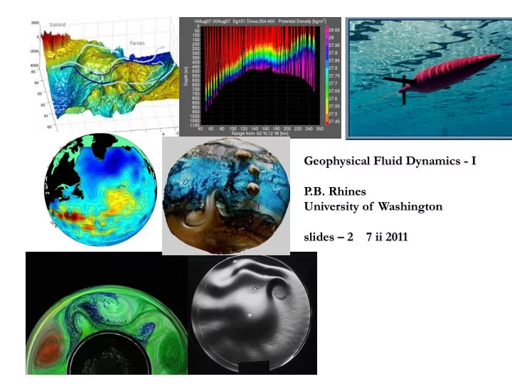
Geophysical Fluid Dynamics - I P.B. Rhines University of Washington slides – 2 7 ii 2011
SLIDE 2
wintertime sea level pressure (very similar to dynamic height Z at 1000 Hpa); note major lows over the northern Atlantic and Pacific in winter. Blue= low pressure, red= high pressure (not T!)
SLIDE 3
black contours are 500 Hpa dyn. height Z. Note the shift of the low pressure center westward with increasing height.
SLIDE 4
A snapshot of the jetstream (as seen at 500 Hpa) when we were in Greenland trying to launch Seagliders from a small boat 100 km offshore. Gale force winds were supplied by fast-moving lows arriving from the Great Lakes, where a deep trough in the jetstream was stationary for some days. Three hurricanes reached Greenland in the 4 weeks prior to launch, energizing when they passed beneath the jetstream
SLIDE 5
Case study animation: Dec 2004
SLIDE 6
temperature at 850 HPa: cold air outbreaks sweep southward from the Arctic; relating such strong movement of cold air to the dynamic height, velocity etc using NCEP data would be very interesting.
SLIDE 7
- Within the last 5 years we have, for
the first time, a global observing system for the oceans, based on satellite altimetry (later SWOT) (currently two US satellites and EU satellites), surface drifting buoys and ~ 3000 subsurface drifting ARGO floats.
- In addition, observations with new
technologies are targeting special regions: robotic gliders, smart profiling moorings, RAFOS floats, articulate chemical tracers (purposefully introduced (SF6, and inadvertant (tritium, CFCs, 129I))
Ocean observations: circulation models,
- bservations, lab experiments have reached
a new level of accuracy…and actually can now talk to one another!
SLIDE 8 Satellite altimetry, with a repeat cycle of typically 10 days for each satellite, gives us synoptic (time- resolved) observations of the ocean surface elevation, hence subsurface pressure, hence geostrophic
- circulation. It does not see the time-averaged pressure associated with the time-mean circulation but
this background field is more and more accurately being reconstructed. In part the GRACE twin gravity satellites which are doing this, but there are many other strong constraints (surface drifting buoys, hydrography) being applied. Thus you do not see the great ocean gyres and jets of the time-
- mean. These mean fields are shown in a later slide. Below we see a snapshot of the global sea-
surface elevation, part of an animation from 1992 to present. A single satellite resolves coarsely, two satellites more finely, the large-length-scale end of the energy-containing eddy spectrum The dimples and pimples march westward almost everywhere on
- Earth. The only significant eastward propagation is seen in the Antarctic Circumpolar Current (the
greatest of all ocean currents, in the Southern Ocean. Even the eastward-flowing Gulf Stream and Kuroshio jets fail to force much eastward phase progression (they are ‘rivers meandering’ eastward).
Chelton et al. 2007 Geophys Res. Lett.
SLIDE 9
SLIDE 10
Time averaged surface circulation of the world ocean deduced from surface drifting buoys, satellite altimetry and ARGO float hydrography. Given as surface displacement in cm. This is the mean upon which the eddy variability shown in the previous slides is riding.
SLIDE 11
Erika Dan section (temperature) 60N (Worthington- Wright Atlas)
SLIDE 12 contours of the Earth’s geopotential field,Ф (gravity and centrifugal effects), for a point-mass approximation to
SLIDE 13
Earth’s geopotential field, Φ equatorial plane rotation vector km km
SLIDE 14
SLIDE 15
SLIDE 16
SLIDE 17
SLIDE 18
SLIDE 19
SLIDE 20
SLIDE 21
SLIDE 22
SLIDE 23 Taylor Proudman effect: the surface elevation above the plastic-grid mountain (far beneath the fluid surface). Constant density, rotating fluid seen with altimetry, GFD lab
- UW. The amplitude of the hills and valleys seen here is
about 1 micron (10-6 m)
SLIDE 24
Free surface elevation…a dome above a submerged mountain which you cannot see directly
SLIDE 25
SLIDE 26
Inertial waves generated by an oscillating ball at the free surface (these are internal waves somewhat different from the hydrostatic long gravity/ inertial waves we have looked at)…but related.
SLIDE 27
SLIDE 28
SLIDE 29
SLIDE 30
SLIDE 31 SSurface elevation when fluid is sweeping cyclonically round the cylindrical
small mountain at 2 o’clock produces a set of jet streams and Rossby waves The center of the basin is the North Pole and thus the mean fluid flow is eastward about the Pole
SLIDE 32 Particle streaklines superimposed