Geometric Reconstruction in Bioluminescence Tomography (BLT) - PowerPoint PPT Presentation

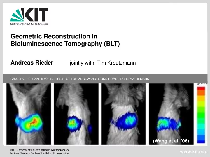
Geometric Reconstruction in Bioluminescence Tomography (BLT) Andreas Rieder jointly with Tim Kreutzmann FAKULT ¨ AT F ¨ UR MATHEMATIK – INSTITUT F ¨ UR ANGEWANDTE UND NUMERISCHE MATHEMATIK (Wang et al. ’06) KIT – University of the State of Baden-W¨ urttemberg and www.kit.edu National Research Center of the Helmholtz Association

Overview Mathematical model Inverse problem: formulation & uniqueness Inverse problem: reformulation & stabilization Gradient of the minimization functional Numerical experiments in 2D Summary 2 / 32 � Andreas Rieder – Geometric Reconstruction in Bioluminescence Tomography c CBM 2013, Rio de Janeiro

Mathematical ⊲ model Inverse problem: formulation & uniqueness Inverse problem: reformulation & stabilization Gradient of the mini- Mathematical model mization functional Numerical experi- ments in 2D Summary 3 / 32 � Andreas Rieder – Geometric Reconstruction in Bioluminescence Tomography c CBM 2013, Rio de Janeiro

The (stationary) radiative transfer equation (RTE) (Boltzmann transport equation) Let u ( x, θ ) be the photon flux (radiance) in direction θ ∈ S 2 about x ∈ Ω ⊂ R 3 . Then, � η ( θ · θ ′ ) u ( x, θ ′ )d θ ′ + q ( x, θ ) θ · ∇ u ( x, θ ) + µ ( x ) u ( x, θ ) = µ s ( x ) S 2 u ( x, θ ) = g − ( x, θ ) , x ∈ ∂ Ω , n ( x ) · θ ≤ 0 � g ( x ) = 1 n ( x ) · θu ( x, θ )d θ, x ∈ ∂ Ω 4 π S 2 where µ = µ s + µ a and µ s / µ a scattering/absorption coefficients � S 2 η ( θ · θ ′ )d θ ′ = 1 ) η scattering kernel ( q source term µ s = 0 : RTE yields integral eqs. of transmission and emission tomography (F. Natterer & F. W¨ ubbeling, Math. Methods in Image Reconstr., SIAM, ’01) 4 / 32 � Andreas Rieder – Geometric Reconstruction in Bioluminescence Tomography c CBM 2013, Rio de Janeiro

Diffusion approximation: setting Assume that u ( x, θ ) = u 0 ( x ) + 3 θ · u 1 ( x ) where � � u 0 ( x ) = 1 u 1 ( x ) = 1 θu ( x, θ )d θ ∈ R 3 . u ( x, θ )d θ ∈ R and 4 π 4 π S 2 S 2 By the Funk-Hecke theorem, � θη ( θ · θ ′ )d θ = η θ ′ S 2 � θ ′ · θ η ( θ · θ ′ )d θ is the scattering anisotropy. where η = S 2 5 / 32 � Andreas Rieder – Geometric Reconstruction in Bioluminescence Tomography c CBM 2013, Rio de Janeiro

Diffusion approximation: derivation Integrate RTE over S 2 , multiply RTE by θ , integrate again, and assume g − ( x, θ ) = g − ( x ) . Then, � −∇ · ( D ∇ u 0 ) + µ a u 0 = q 0 := 1 q ( · , θ )d θ, 4 π S 2 u 0 + 2 D∂ n u 0 = g − on ∂ Ω , D∂ n u 0 = − g on ∂ Ω , where 1 D = 3( µ − ηµ s ) is the diffusion coefficient (reduced scattering coefficient). 6 / 32 � Andreas Rieder – Geometric Reconstruction in Bioluminescence Tomography c CBM 2013, Rio de Janeiro

Diffusion approximation: final equation Change of notation: u = u 0 , q = q 0 , µ = µ a , and g = − g . The photon density u obeys the BVP −∇ · ( D ∇ u ) + µu = q in Ω , u + 2 D∂ n u = g − on ∂ Ω . The measurements are given by D∂ n u = g on ∂ Ω . Assume g − = 0 (no photons penetrate the object from outside). 7 / 32 � Andreas Rieder – Geometric Reconstruction in Bioluminescence Tomography c CBM 2013, Rio de Janeiro

Mathematical model Inverse problem: formulation & ⊲ uniqueness Inverse problem: reformulation & stabilization Gradient of the mini- mization functional Inverse problem: formulation & uniqueness Numerical experi- ments in 2D Summary 8 / 32 � Andreas Rieder – Geometric Reconstruction in Bioluminescence Tomography c CBM 2013, Rio de Janeiro

Inverse problem of BLT (in the diffusive regime) Define the (linear) forward operator A : L 2 (Ω) → H − 1 2 ( ∂ Ω) , q �→ D∂ n u , where u solves the BVP with g − = 0 : −∇ · ( D ∇ u ) + µu = q in Ω , u + 2 D∂ n u = 0 on ∂ Ω . BLT Problem : Given g ∈ R ( A ) , find a source q ∈ L 2 (Ω) satisfying Aq = g. 9 / 32 � Andreas Rieder – Geometric Reconstruction in Bioluminescence Tomography c CBM 2013, Rio de Janeiro

Null Space of A Lemma (Wang, Li & Jiang ’04, Kreutzmann ’13) : There is an isomorphism Φ: H 1 (Ω) → H 1 (Ω) ′ such that � � H 1 ∩ L 2 (Ω) . N ( A ) = Φ 0 (Ω) If D ∈ W 1 , ∞ then � � H 1 0 (Ω) ∩ H 2 (Ω) N ( A ) = Φ . Proof: Define Φ: H 1 (Ω) → H 1 (Ω) ′ , u �→ (Φ u )( v ) = a ( u, v ) where � � � � d x + 1 a ( u, v ) = D ∇ u · ∇ v + µuv uv d s. 2 Ω ∂ Ω 10 / 32 � Andreas Rieder – Geometric Reconstruction in Bioluminescence Tomography c CBM 2013, Rio de Janeiro

Singular Functions of A : L 2 (Ω 0 ) → L 2 ( ∂ Ω) σ 1 = 0.34221 σ 2 = 0.2932 σ 3 = 0.23248 σ 4 = 0.17673 5 5 5 5 0.2 0.2 0.2 −0.1 0 −0.2 0 0 0 0 0 0 −0.3 −0.2 −0.2 −0.2 −5 −5 −5 −5 −0.4 −0.4 M −8 −6 −4 −8 −6 −4 −8 −6 −4 −8 −6 −4 σ 5 = 0.1296 σ 6 = 0.096659 σ 7 = 0.070445 σ 8 = 0.04619 0.4 5 5 5 5 0.2 0.2 0.2 0.2 L H L 0 0 0 0 0 0 0 0 −0.2 −0.2 −0.2 −0.2 −5 −5 −5 −5 −0.4 −8 −6 −4 −8 −6 −4 −8 −6 −4 −8 −6 −4 σ 9 = 0.035356 σ 10 = 0.021841 σ 11 = 0.013265 σ 12 = 0.0089158 B 0.4 0.4 0.4 5 5 5 5 0.2 0.2 0.2 0.2 0 0 0 0 0 0 0 0 −0.2 −0.2 −0.2 −5 −5 −5 −5 −0.2 −0.4 −0.4 −8 −6 −4 −8 −6 −4 −8 −6 −4 −8 −6 −4 11 / 32 � Andreas Rieder – Geometric Reconstruction in Bioluminescence Tomography c CBM 2013, Rio de Janeiro

Can we restore uniqueness by a priori information? Consider, for instance, q = λχ S where λ ≥ 0 is a constant and S ⊂ Ω . 12 / 32 � Andreas Rieder – Geometric Reconstruction in Bioluminescence Tomography c CBM 2013, Rio de Janeiro

Can we restore uniqueness by a priori information? Consider, for instance, q = λχ S where λ ≥ 0 is a constant and S ⊂ Ω . Lemma (Wang, Li & Jiang ’04) : There exist z ∈ Ω , λ 1 � = λ 2 and r 1 � = r 2 such that A ( λ 1 χ B 1 ) = A ( λ 2 χ B 2 ) with B k = B r k ( z ) . 12 / 32 � Andreas Rieder – Geometric Reconstruction in Bioluminescence Tomography c CBM 2013, Rio de Janeiro

Mathematical model Inverse problem: formulation & uniqueness Inverse problem: reformulation & ⊲ stabilization Reformulation Tikhonov -like Inverse problem: regularization Existence of a reformulation & stabilization minimizer & stability Regularization property Gradient of the mini- mization functional Numerical experi- ments in 2D Summary 13 / 32 � Andreas Rieder – Geometric Reconstruction in Bioluminescence Tomography c CBM 2013, Rio de Janeiro

Reformulation I � Ansatz: q = λ i χ S i where S i ⊂ Ω , λ i ∈ [ λ i , λ i ] = Λ i , and I ∈ N . i =1 For the ease of presentation: I = 1 . Define the nonlinear operator L 2 ( ∂ Ω) , F : Λ × L → ( λ, S ) �→ D∂ n u | ∂ Ω where L is the set of all measurable subsets of Ω . Note: F ( λ, S ) = λAχ S BLT Problem : Given measurements g , find an intensity λ ∈ Λ and a domain S ∈ L such that F ( λ, S ) = g. 14 / 32 � Andreas Rieder – Geometric Reconstruction in Bioluminescence Tomography c CBM 2013, Rio de Janeiro

Tikhonov-like regularization Minimize J α ( λ, S ) = 1 2 � F ( λ, S ) − g � 2 L 2 + α Per( S ) over Λ × L where α > 0 is the regularization parameter and Per( S ) is the perimeter of S : Per( S ) = | D( χ S ) | , with | D( · ) | denoting the BV -semi-norm (Ramlau & Ring ’07, ’10) . AG Sahin, Univ. Mainz 15 / 32 � Andreas Rieder – Geometric Reconstruction in Bioluminescence Tomography c CBM 2013, Rio de Janeiro

Existence of a minimizer & stability Theorem: For all α > 0 and g ∈ L 2 ( ∂ Ω) there exists a minimizer ( λ ∗ , S ∗ ) ∈ Λ × L , that is, J α ( λ ∗ , S ∗ ) ≤ J α ( λ, S ) for all ( λ, S ) ∈ Λ × L . Theorem: Let g n → g in L 2 as n → ∞ and let ( λ n , S n ) minimize α ( λ, S ) = 1 2 � F ( λ, S ) − g n � 2 J n L 2 + α Per( S ) over Λ × L . Then there exists a subsequence { ( λ n k , S n k ) } k converging to a minimizer ( λ ∗ , S ∗ ) ∈ Λ × L of J α in the sense that � λ n k χ S nk − λ ∗ χ S ∗ � L 2 → 0 as k → ∞ . Furthermore, every convergent subsequence of { ( λ n , S n ) } n converges to a minimizer of J α . 16 / 32 � Andreas Rieder – Geometric Reconstruction in Bioluminescence Tomography c CBM 2013, Rio de Janeiro

Regularization property Theorem: Let g be in range( F ) and let δ �→ α ( δ ) where δ 2 α ( δ ) → 0 and α ( δ ) → 0 as δ → 0 . In addition, let { δ n } n be a positive null sequence and { g n } n such that � g n − g � L 2 ≤ δ n . Then, the sequence { ( λ n , S n ) } of minimizers of J n α ( δ n ) possesses a sub - sequence converging to a solution ( λ + , S + ) where S + = arg min { Per( S ) : S ∈ L s.t. ∃ λ ∈ Λ with F ( λ, S ) = g } . Furthermore, every convergent subsequence of { ( λ n , S n ) } n converges to a pair ( λ † , S † ) with above property. 17 / 32 � Andreas Rieder – Geometric Reconstruction in Bioluminescence Tomography c CBM 2013, Rio de Janeiro