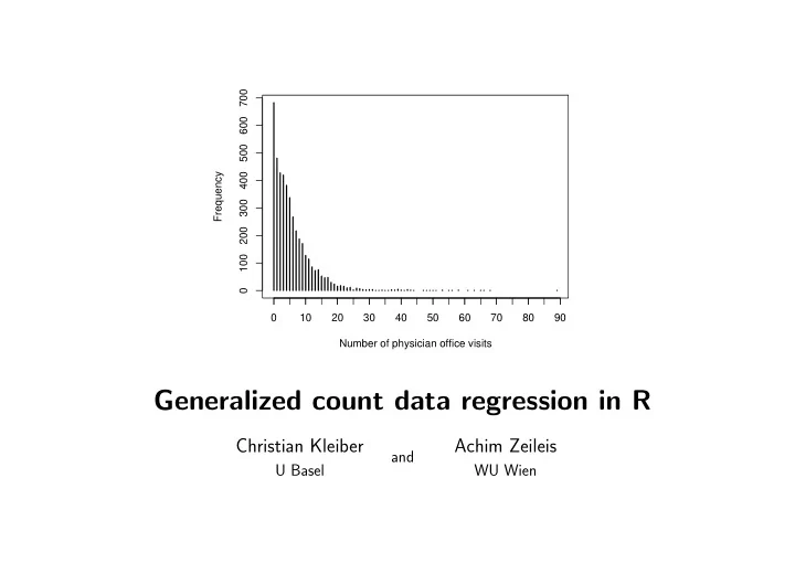
Generalized count data regression in R Christian Kleiber Achim - - PowerPoint PPT Presentation

Number of physician office visits Frequency 100 200 300 400 500 600 700 10 20 30 40 50 60 70 80 90

Generalized count data regression in R

Christian Kleiber

U Basel and

Achim Zeileis

WU Wien

Outline

• Introduction
• Regression models for count data
• Zero-inflation models
• Hurdle models
• Generalized negative binomial models
• Further extensions

C Kleiber

2

U Basel

Introduction

• Classical count data models (Poisson, NegBin) often not flexible enough for applica-

tions in economics and the social sciences.

• Typical problems include overdispersion and excess zeros.

Also relevant in e.g. fisheries research, medical sciences (DMF teeth index) etc.

• Zero-inflation and hurdle models (Mullahy, J. Econometrics 1986, Lambert, Techno-

metrics 1992) address excess zeros, implicitly also overdispersion. Recent paper on implementation in R: Zeileis, Kleiber and Jackman (2008): Regression models for count data in R. J. Sta- tistical Software, 27(8). URL http://www.jstatsoft.org/v27/i8/

• Generalizations of NegBin have more flexible variance function or additional source of

heterogeneity via regressors in shape parameter.

C Kleiber

3

U Basel

Regression models for count data

Classifications:

• Classical count data models:

– Poisson regression – Negative binomial regression (including geometric regression) – Quasi-Poisson regression

• Generalized count data models:

– Zero-inflation models – Hurdle models – NegBin-P model – heterogeneous NegBin model (NB-H)

• Single-index models: Poisson, quasi-Poisson, geometric, negative binomial, NB-P
• Multiple-index models: zero-inflation models, hurdle models, NB-H

C Kleiber

4

U Basel

Regression models for count data

Count data models in R: (incomplete list!)

• stats: Poisson and quasi-Poisson models via glm()
• MASS: negative binomial and geometric regression via glm.nb()
• pscl: zero-inflation and hurdle models via zeroinfl() and hurdle()
• AER: testing for equidispersion via dispersiontest()
• flexmix: finite mixtures of Poissons via flexmix()
• gamlss: Poisson-inverse Gaussian (PIG) regression via gamlss()

C Kleiber

5

U Basel

Regression models for count data

Generalized linear models are defined by 3 elements:

• Linear predictor ηi = x⊤

i β through which µi = E(yi|xi) depends on vectors xi of

• bservations and β of parameters.
• Distribution of dependent variable yi|xi is linear exponential family

f(y; θ, φ) = exp yθ − b(θ) φ + c(y; φ)

• .
• Expected response µi and linear predictor ηi are related by monotonic transformation

g(µi) = ηi, called link function.

C Kleiber

6

U Basel

Regression models for count data

• Poisson model:

f(y; µ) = exp(−µ) · µy y! , y = 0, 1, 2, . . .

• Negative binomial model:

f(y; µ, θ) = Γ(y + θ) Γ(θ) · y! · µy · θθ (µ + θ)y+θ, y = 0, 1, 2, . . .

• Canonical link is g(µ) = log(µ) for both.
• NegBin is GLM only for fixed θ. Special case: geometric distribution for θ = 1.

C Kleiber

7

U Basel

Regression models for count data

Example: (US National Medical Expenditure Survey [NMES] data for 1987/88) Available as NMES1988 in package AER (Kleiber and Zeileis 2008). Originally taken from Deb and Trivedi (J. Applied Econometrics 1997). n = 4406 individuals, aged 66 and over, covered by Medicare Objective: model demand for medical care – here defined as number of physician office visits – in terms of covariates. Variables: visits – number of physician office visits (response) hospital – number of hospital stays health – self-perceived health status chronic – number of chronic conditions gender – gender school – number of years of education insurance – private insurance indicator

C Kleiber

8

U Basel

Regression models for count data

Number of physician office visits Frequency 100 200 300 400 500 600 700 10 20 30 40 50 60 70 80 90

C Kleiber

9

U Basel

Zero-inflation models

A mixture of point mass at zero I{0}(y) and count distribution fcount(y; x, β): fzeroinfl(y; x, z, β, γ) = π · I{0}(y) + (1 − π) · fcount(y; x, β)

• Probability of observing zero count is inflated with probability π.
• More recent applications have π = fzero(0; z, γ).

Unobserved probability π is modelled by binomial GLM π = g−1(z⊤γ).

• Regression equation for the mean is (using canonical [= log] link)

µi = πi · 0 + (1 − πi) · exp(x⊤

i β),

• Vectors of regressors zi and xi need not be distinct.
• Inference for (β, γ, θ) by ML. θ is treated as nuisance parameter.

C Kleiber

10

U Basel

Zero-inflation models

In R:

• Package pscl has function zeroinfl()
• Typical call looks like

R> dt_zinb <- zeroinfl(visits ~ . | + hospital + chronic + insurance + school + gender, + data = dt, dist = "negbin")

• Count part specified by dist argument, using canonical [= log] link.
• Binary part defaults to link = "logit", other links also available.
• Optimization via optim(). Otherweise GLM building blocks are reused.
• Methods include coef(), fitted(), logLik(), predict(), summary(), vcov().

C Kleiber

11

U Basel

Zero-inflation models

Call: zeroinfl(formula = visits ~ . | hospital + chronic + insurance + school + gender, data = dt, dist = "negbin") Count model coefficients (negbin with log link): Estimate Std. Error z value Pr(>|z|) (Intercept) 1.19372 0.05666 21.07 < 2e-16 hospital 0.20148 0.02036 9.90 < 2e-16 healthpoor 0.28513 0.04509 6.32 2.6e-10 healthexcellent -0.31934 0.06040

• 5.29

1.2e-07 chronic 0.12900 0.01193 10.81 < 2e-16 gendermale

• 0.08028

0.03102

• 2.59

0.0097 school 0.02142 0.00436 4.92 8.8e-07 insuranceyes 0.12586 0.04159 3.03 0.0025 Log(theta) 0.39414 0.03503 11.25 < 2e-16

C Kleiber

12

U Basel

Zero-inflation models

Zero-inflation model coefficients (binomial with logit link): Estimate Std. Error z value Pr(>|z|) (Intercept)

• 0.0468

0.2686

• 0.17

0.8615 hospital

• 0.8005

0.4208

• 1.90

0.0571 chronic

• 1.2479

0.1783

• 7.00

2.6e-12 insuranceyes

• 1.1756

0.2201

• 5.34

9.3e-08 school

• 0.0838

0.0263

• 3.19

0.0014 gendermale 0.6477 0.2001 3.24 0.0012 Theta = 1.483 Number of iterations in BFGS optimization: 28 Log-likelihood: -1.21e+04 on 15 Df

C Kleiber

13

U Basel

Hurdle models

Hurdle model combines

• Count part fcount(y; x, β) (count left-truncated at y = 1)
• Zero hurdle part fzero(y; z, γ) (count right-censored at y = 1)

fhurdle(y; x, z, β, γ) =

• fzero(0; z, γ)

if y = 0, (1 − fzero(0; z, γ)) ·

fcount(y;x,β) 1−fcount(0;x,β)

if y > 0 Inference for parameters (β, γ, θ) by ML. θ is treated as nuisance parameter. Logit and censored geometric models as hurdle part both lead to same likelihood, and thus to identical estimates. If same regressors xi = zi are used one can test β = γ – is hurdle needed or not?

C Kleiber

14

U Basel

Hurdle models

In R:

• Package pscl has function hurdle()
• Typical call is

R> dt_hurdle <- hurdle(visits ~ . | + hospital + chronic + insurance + school + gender, + data = dt, dist = "negbin")

• Count part specified by dist argument, using canonical [= log] link.
• Binary part defaults to zero.dist = "binomial" with link = "logit", other

links and distributions also available.

• Optimization via optim(). Otherweise GLM building blocks are reused.
• Methods include coef(), fitted(), logLik(), predict(), summary(), vcov().

C Kleiber

15

U Basel

Hurdle models

Call: hurdle(formula = visits ~ . | hospital + chronic + insurance + school + gender, data = dt, dist = "negbin") Count model coefficients (truncated negbin with log link): Estimate Std. Error z value Pr(>|z|) (Intercept) 1.19770 0.05897 20.31 < 2e-16 hospital 0.21190 0.02140 9.90 < 2e-16 healthpoor 0.31596 0.04806 6.57 4.9e-11 healthexcellent -0.33186 0.06609

• 5.02

5.1e-07 chronic 0.12642 0.01245 10.15 < 2e-16 gendermale

• 0.06832

0.03242

• 2.11

0.035 school 0.02069 0.00453 4.56 5.0e-06 insuranceyes 0.10017 0.04262 2.35 0.019 Log(theta) 0.33325 0.04275 7.79 6.5e-15

C Kleiber

16

U Basel

Hurdle models

Zero hurdle model coefficients (binomial with logit link): Estimate Std. Error z value Pr(>|z|) (Intercept) 0.0159 0.1378 0.12 0.90788 hospital 0.3184 0.0911 3.50 0.00047 chronic 0.5478 0.0436 12.57 < 2e-16 insuranceyes 0.7457 0.1003 7.43 1.1e-13 school 0.0571 0.0119 4.78 1.7e-06 gendermale

• 0.4191

0.0875

• 4.79

1.7e-06 Theta: count = 1.396 Number of iterations in BFGS optimization: 16 Log-likelihood: -1.21e+04 on 15 Df

C Kleiber

17

U Basel

Generalized negative binomial models

NegBin-P model: (Winkelmann and Zimmermann 1991, Greene 2008) Negative binomial in standard parametrization has variance function Var(yi|xi) = µi

• 1 + 1

θµi

• Special case of

Var(yi|xi) = µi

• 1 + 1

θµP −1

i

• Common versions are P = 1, 2, called NB1 and NB2.

Can also estimate P, this gives NB-P model.

C Kleiber

18

U Basel

Generalized negative binomial models

NegBin-H model: (Greene 2007) Further generalization to multiple index model via Var(yi|xi) = µi

• 1 + 1

θi µP −1

i

• with θi = exp (z⊤

i γ).

R implementation of NB-P and NB-H by D. Cueni (M.S. thesis, U Basel 2008). Optimization via nlminb(). Programs allow for fixing P, thus enabling NB1 regression.

C Kleiber

19

U Basel

Generalized negative binomial models

Results for 4 models: R> logLik(dt_nb2) ’log Lik.’ -12171 (df=9) R> logLik(dt_hurdle) ’log Lik.’ -12090 (df=15) R> logLik(dt_nbp) ’log Lik.’ -12135 (df=10) R> logLik(dt_nbh) ’log Lik.’ -12098 (df=15)

C Kleiber

20

U Basel

Generalized negative binomial models

0.00 0.05 0.10 0.15

Actual vs Estimated Frequencies

Values Frequency 2 4 6 8 10 12 14 16 18 20 22

C Kleiber

21

U Basel

Further extensions

Welcome additions:

• more on multivariate count data models (bivpois has bivariate Poisson models)
• more on finite mixtures (flexmix has finite mixtures of Poissons, but not of NegBins).
• count models for panels (to some extent available in lme4, glmmML, . . . )
• further Poisson mixtures
• count models with endogeneity, selectivity, . . .

C Kleiber

22

U Basel