Fractal attractors in skew products systems III: Hausdorff dimension - PowerPoint PPT Presentation

Fractal attractors in skew products systems III: Hausdorff dimension of Weierstrass graphs Tobias J¨ ager 4th Bremen Winter School Dynamics, Chaos and Applications 14-18 March 2016

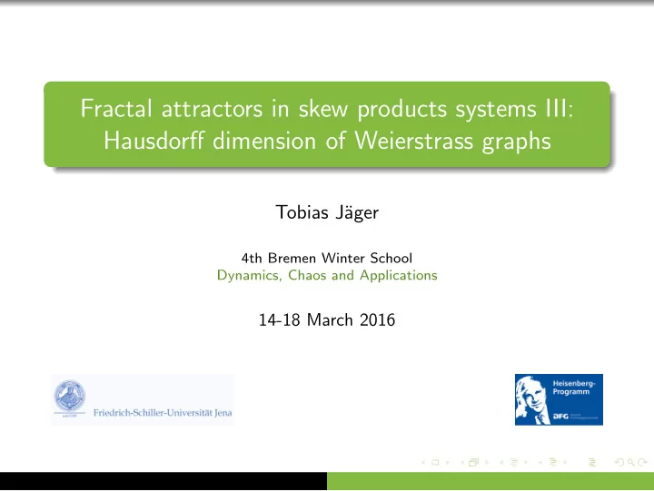
The Weierstrass graph Graph of the Weierstrass function. (Source: Wikipedia)

The Weierstrass graph The Weierstrass function is defined as ∞ λ n cos(2 π b n θ ) � ϕ ( θ ) = n =0 with λ ∈ (0 , 1) and b > 1 /λ . It is an invariant graph of the skew product system � � bx mod 1 , x − cos(2 πθ ) F : T 1 × R → T 1 × R , ( θ, x ) �→ . λ Theorem (Baranski/Barany,Romanowska 2014, Shen 2015) The Hausdorff dimension of the Weierstrass graph equals D = 2 + log λ log b . We consider the case b = 2 and λ ∈ (1 / 2 , 1).

Invertible extension Let τ : T 2 → T 2 , ( ϑ, θ ) �→ (2 ϑ, θ/ 2 + k ( ϑ ) / 2) be the standard baker’s map, where k ( ϑ ) = 0 if ϑ ∈ [0 , 1 / 2) and k ( ϑ ) = 1 otherwise. Then an invertible extension of F is given by � τ − 1 ( ϑ, θ ) , x − cos(2 πθ ) � ˜ F ( ϑ, θ, x ) = . λ If we let ξ = ( ϑ, θ ) and consider the inverse of ˜ F , we obtain T : T 2 × R → T 2 × R , ( ξ, x ) �→ ( τ ( ξ ) , λ x + cos(2 π ( θ/ 2 + k ( ϑ ) / 2))) . This map preserves the foliations into horizontal and vertical circles, which will allow to ignore the discontinuities at ϑ = 0 , 1 / 2.

Invariant manifolds As in the previous examples, there exists a strong stable foliation. Since the stable manifolds in the base are just vertical lines, these can be represented as smooth graphs of functions ξ, x : T 1 → R θ ′ �→ γ s γ s , ξ, x ( θ ) . The ϑ -coordinate is omitted in the representation, so the strong stable manifolds W s ( ξ, x ) are viewed as subsets of the ( θ, x )-section at ϑ . Note that the unstable manifolds are just horizontal lines, and again the weak stable manifolds are the fibres.

Invariant vector fields T is partially hyperbolic with Lyapunov exponents log 2, log(1 / 2) and log λ . The invariant vector fields corresponding to log b and log λ are just the constant vectors (1 , 0 , 0) and (0 , 0 , 1). For the strong stable invariant subspace V ( ϑ, θ, x ) = (0 , 1 , v ( ϑ, θ, x )), we obtain the following recursive formula. DT ( ϑ, θ, x ) · V ( ϑ, θ, x )       2 0 0 0 0  = 0 1 / 2 0  · 1 1 / 2 =     0 g ( ϑ ) λ v ( ϑ, θ ) v ( τ ( ϑ, θ )) / 2 where g ( θ, ϑ ) = ∂ θ cos (2 π ( θ/ 2 + k ( ϑ ) / 2)).

The strong stable subspaces We thus obtain g ( ϑ, θ ) + λ v ( ϑ, θ ) = v ( τ ( ϑ, θ )) / 2 and hence a solution ∞ � α n g ( τ n − 1 ( ϑ, θ )) v ( ϑ, θ ) = − n =1 ∞ α n sin(2 πθ n ) � = 2 π n =1 where α = 1 / 2 λ and θ n = π 2 ◦ τ n ( θ, ϑ ). The latter is the curve ϕ ( θ, ϑ ) from Tsujii’s model, so that for fixed ϑ the distribution of v ( ϑ, . ) is absolutely continuous with respect to Lebesgue.

Pointwise and Hausdorff dimension of measures Given a measure µ on some metric space Y , the pointwise dimension of µ in y ∈ Y is given by log µ ( B ε ( x )) d ( µ, y ) = lim . log ε ε → 0 If the pointwise dimension exists and equals d ≥ 0 µ -almost everywhere, then Dim H ( µ ) = A ⊆ Y , µ ( A ) > 0 Dim H ( A ) = d . inf Thus, in our situation, we need to show that d ( µ, ξ ) = 2 + log λ log b µ -almost everywhere.

Ledrappier-Young Theory For fixed ϑ , the measure µ on the graph of W can be projected along the strong stable foliation to a vertical line L . Denote the resulting measure by ν ϑ . Then, as in the decomposition of measures on product spaces, there exist conditional measures µ ( ϑ,θ, x ) supported on the strong stable leaves of ( θ, x ) in the ϑ -fibre. Ledrappier-Young theory for the dimensions of ergodic measures of (partially hyperbolic) diffeomorphisms now states that the pointwise dimensions exist and are constant almost surely for all these measures and we have Dim H ( µ ) = Dim H ( µ ξ, x ) + Dim H ( ν ϑ ) , Dim H ( µ ξ, x ) log 2 = log 2 + log λ Dim H ( ν ϑ ) . Together, this means that � 1 + log λ � Dim H ( µ ) = 1 + Dim H ( ν ϑ ) . log 2

Marstrand Projection The measure ν ϑ is absolutely continuous, and hence has dimension 1, if the tangent vectors v ( ., θ ) of the strong stable manifolds, as a function of ϑ , have an absolutely continuous distribution. (Nonlinear Marstrand projection, sketch proof by Ledrappier, proof by Atsuya Otani). Altogether, we obtain Dim H (Φ) = 2 + log λ log 2 for all parameters λ which allow to apply Tsujii’s argument. Shen has recently shown that this are all λ > 1 / 2.