For example, graph the following parametric functions for 2 t 2 - - PDF document

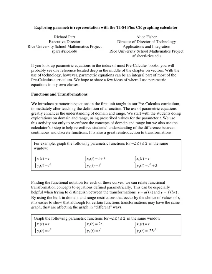
Exploring parametric representation with the TI-84 Plus CE graphing calculator Richard Parr Executive Director Rice University School Mathematics Project rparr@rice.edu Alice Fisher Director of Director of Technology Applications and Integration Rice University School Mathematics Project afisher@rice.edu If you look up parametric equations in the index of most Pre-Calculus books, you will probably see one reference located deep in the middle of the chapter on vectors. With the use of technology, however, parametric equations can be an integral part of most of the Pre-Calculus curriculum. We hope to share a few ideas of where I use parametric equations in my own classes. Functions and Transformations We introduce parametric equations in the first unit taught in our Pre-Calculus curriculum, immediately after teaching the definition of a function. The use of parametric equations greatly enhances the understanding of domain and range. We start with the students doing explorations on domain and range, using prescribed values for the parameter t. We use this activity not only to re-enforce the concepts of domain and range but we also use the calculator’s t-step to help re-enforce students’ understanding of the difference between continuous and discrete functions. It is also a great reintroduction to transformations. Finding the functional notation for each of these curves, we can relate functional transformation concepts to equations defined parametrically. This can be especially helpful when trying to distinguish between the transformations ( ) y af x  and y f bx  ( ) . By using the built in domain and range restrictions that occur by the choice of values of t, it is easier to show that although for certain functions transformations may have the same graph, they are affecting the graph in “different” ways. For example, graph the following parametric functions for 2 2 t    in the same window:

1 2 1

( ) ( ) x t t y t t       

2 2 2

( ) 3 ( ) x t t y t t        

3 2 3

( ) ( ) 3 x t t y t t         Graph the following parametric functions for 2 2 t    in the same window

1 2 1

( ) ( ) x t t y t t       

2 2 2

( ) 2 ( ) x t t y t t       

3 2 3

( ) ( ) .25 x t t y t t       

Inverses We would feel lost trying to teach the concept of the inverse of a function without using parametric representation. After starting with functional representations of one-to-one functions we move to using parametric equations for both one-to one and non one-to-one

• functions. The idea of “flipping” the x and y equations to create the inverse

parametrically makes sense to the students. We let the students discover the idea of restricting a domain of a function so that it has a functional inverse, and what makes a “good” restriction. This is especially important when teaching the inverses of the trigonometric functions. Introduction to Trigonometry After defining the x and y coordinates of the unit circle in terms of sine and cosine, it is easy to develop the idea of a parametrically defined unit circle. It is nice to show the “unwrapping” of the circle to create the sine graph. Graph the following in the same window for 4 4 t    .

1 2 1

( ) ( ) x t t y t t       

2 2 2

( ) ( ) x t t y t t        The graphs represent the function

2

( ) f x x  and its inverse. Now restrict t so that the inverse is a function. Graph the following for 0 2 t    using a t-step of 24  . Use a window of 1.5 6.5 x    and 2.67 2.67 y    .

1 1

( ) cos( ) ( ) sin( ) x t t y t t     

2 2

( ) ( ) sin( ) x t t y t t     

Conic Sections The Pythagorean trigonometric identities allow for easy parametric representation of ellipses and hyperbolas. Parabolas are most easily represented without the use of trigonometry. Ellipses A comparison of the Pythagorean identity: cos sin

2 2

1 t t   and a standard form for the equation of an ellipse :

  x h a y k b    

2 2 2 2

1 ( ) allows for two simple substitutions : cos ( )

2 2 2

t x h a   and sin ( )

2 2 2

t y k b   Solving these two equations for x and y yields a pair of parametric equations: x a t h   cos y b t k   sin A few personal comments are important at this point: I chose substitutions I did to reinforce the use of x and y coordinates of a unit circle to represent sine and cosine respectively. In using this method I am de-emphasizing the idea that “a” corresponds to the major axis, etc. I focus on the idea that “a” is a stretch in the x equation and therefore a horizontal stretch. Likewise, “b” is a vertical stretch. I’d just as soon not use the letters “a” and “b” at all, but focus on the major axis being the axis with the “largest” stretch. Some students see a contradiction in the transformation in parametric representation when compared to the Cartesian representation. By re-writing 5 cos 3   t x in the form t x cos 3 5   , I try to show that there is really no contradiction. Re-express 1 4 ) 1 ( 9 ) 5 (

2 2

    y x using parametric equations and graph. Use degree mode and graph in an appropriate square window for 0 360 t   

Hyperbolas By using the Pythagorean identity: sec tan

2 2

1 t t   and a standard form for a hyperbola : 1 ) ( ) (

2 2 2 2

    b k y a h x

• r

1 ) ( ) (

2 2 2 2

    b h x a k y One can derive the following pairs of parametric equations to represent hyperbolas: x a t h   sec x b t h   tan y b t k   tan y a t k   sec (horizontal transverse axis) (vertical transverse axis) In a hyperbola, unlike an ellipse, it makes a difference which trigonometric function corresponds with which variable. Parabolas Parabolas are most easily graphed parametrically without the use of trigonometric

• functions. All non-rotated parabolas can either be written in the form y

f x  ( ) or x f y  ( ). Parametrically, parabolas that can be written y f x  ( )can be graphed using x t  and y f t  ( ) , likewise parabolas that can be represented as x f y  ( ) can be graphed parametrically using x f t  ( ) and y t  . In this case the t-step of the window must be adjusted to include negative values for t or the entire parabola will not appear. Extensions Exploring rotated conic sections is an extension of this work. To do this view a pair of parametric equations as a 2 x 1 vector matrix; ( ) ( ) x t y t       , then left-multiply this matrix by a rotation matrix; [cos 𝜄 − sin 𝜄 sin 𝜄 cos 𝜄 ]. Using the same window settings as before, re-express the equation parametrically to graph the hyperbola ( ) ( ) y x     2 25 1 36 1

2 2

.

The resultant 2 x1 matrix; [cos 𝜄 ∙ 𝑦(𝑢) − sin 𝜄 ∙ 𝑧(𝑢) sin 𝜄 ∙ 𝑦(𝑢) + cos 𝜄 ∙ 𝑧(𝑢)] represents a new pair of parametric equations that rotate the conic q degrees counter- clockwise. Vectors Parametric representation allows for the exploration of two dimensional motion problems, especially those related with projectile motion. By using the parametric equations: ( cos )

• x

v t  

• s

t v at y    ) sin ( 2 1

2

 (Where vo is initial velocity, q is the angle of projection, a is acceleration due to gravity and so is initial height at projection.) One can explore the effects of changing the various parameters. Many calculator games have been developed that use these ideas in situations such as throwing a basketball or javelin, or hitting a baseball. In the same window graph the hyperbola from the previous example and the same hyperbola rotated 45 counter-clockwise. Find an appropriate graphing window and model the motion of an object projected with an initial velocity of 50m/s at an angle of 30 from the horizontal from a height

• f 3 m. Assume that acceleration due to gravity is -9.8m/s2.