First-principle molecular dynamics with ultrasoft pseudopotentials: - - PowerPoint PPT Presentation

First-principle molecular dynamics with ultrasoft pseudopotentials: theory, parallel implementation, applications

• P. Giannozzi

Scuola Normale Superiore di Pisa and Democritos National Simulation Center, Italy

• Ultrasoft Vanderbilt pseudopotentials in first-principle molecular dynamics
• Practical implementation and parallelization
• Applications: biologically relevant molecules

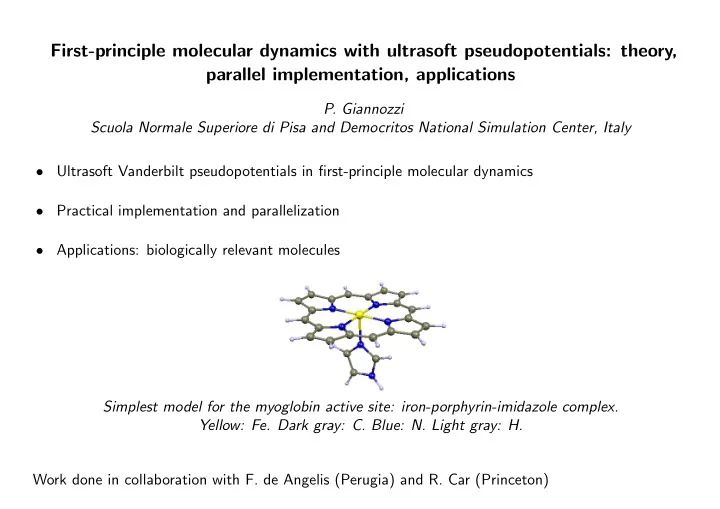
Simplest model for the myoglobin active site: iron-porphyrin-imidazole complex. Yellow: Fe. Dark gray: C. Blue: N. Light gray: H. Work done in collaboration with F. de Angelis (Perugia) and R. Car (Princeton)

Goal: Modellization of biological molecules (and of their reactions) containing transition metal centers. Extended model of the myoglobin active site, including the 13 surrounding residues in a 8A sphere centered around the iron atom, terminated with NH2 groups (332 atoms, 902 electrons). Red: O, other atoms as in previous figure. Interest: respiration, photosynthesis, enzymatic catalysis...

Influence of the protein environment Spin density distribution of the quintet state (S = 2) for the extended model of the myoglobin active site, showing a sizable contribution not localized on the Iron atom

Problems to be addressed:

• high-level theoretical description needed, due to the presence of transition metal atoms
• complex energy landscape: many possible spin states and local minima, not easy to guess from

static (single-point) calculations

• large systems (hundreds of atoms) needed in order to accurately describe the effect of surrounding

environment A powerful tool: First-Principle Molecular Dynamics

• combines forces on atoms from electronic structure with classical Molecular Dynamics simulation

machinery

• forces on atoms are usually obtained from Density-Functional Theory
• a convenient way to perform First-Principle Molecular Dynamics: Car-Parrinello dynamics on both

electronic and nuclear degrees of freedom

Density-Functional Theory The energy is a functional of the charge density n(r): EDF T = F[n(r)] +

• n(r)V (r)dr

that is minimized by the ground-state charge density n(r). Typically solved via Kohn-Sham equations:

• − 2

2m∇2 + V (r) + VH(r) + Vxc(r)

• ψi(r) = ǫiψi(r)

where n(r) =

• i

|ψi(r)|2, ψi|ψj = δij, the Hartree potential VH(r) is: VH(r) = e2

• n(r′)

|r − r′|dr′, and Vxc(r) is a suitable exchange-correlation potential, approximated as a function of n(r) and of its gradient |∇n(r)|.

Forces in Density-Functional Theory Forces acting on nuclei have the simple Hellmann-Feynman form: FI = −∂E({RI}) ∂RI = −

• n(r) ∂V

∂RI dr + ∂EN ∂RI RI = position of I−th nucleus, E({RI}) = EDF T + EN, EN = nuclear electrostatic energy. Structural minimization: find minimum of E({RI}), calculated for the electronic ground-state charge density corresponding to nuclei in positions {RI}. Molecular Dynamics: introduce Lagrangian L = 1 2

• I

MI∇2

RI − E({RI})

generating equations of motions: FI = MI ¨ RI = −∂E({RI}) ∂RI that can be discretized in time using i.e. Verlet algorithm.

Car-Parrinello Molecular Dynamics Introduce fictitious dynamics on the electronic degrees of freedom ψi: L = µ

• i
• | ˙

ψi(r)|2 + 1 2

• I

MI∇2

RI − E({ψi}, {RI})

(µ = fictitious electronic mass), subject to orthonormality constraints ψi|ψj − δij = 0. Generated equations of motion: µ ¨ ψi = −δE δψi +

• ij

Λijψj FI = MI ¨ RI = − ∂E ∂RI where Λij = Lagrange multiplier enforcing the constraints. Electrons are initially brought close to the ground state at fixed nuclei. The combined electronic and nuclear dynamics keeps electrons close to the instantaneous ground state.

Practical Implementation A supercell geometry and the corresponding Plane-Wave (PW) basis set are typically used: r|k + G = 1 √ Ω ei(k+G)·r G = reciprocal lattice vectors of the supercell, Ω = unit cell volume, k = Bloch vector. The Bloch vector can be assumed to be k = 0 and dropped for aperiodic systems (molecules). Expansion of orbitals into PW’s: ψn(r) =

• G

ψn(G) 1 √ Ω eiG·r. A finite PW set is obtained by taking all PW’s up to a given kinetic energy cutoff Ec: 2 2m|G|2 ≤ Ec. The basic operation to be performed is the Fourier Transform.

Norm-Conserving Pseudopotentials Electron-ionic core interactions are represented by a nonlocal norm-conserving pseudopotential (NCPP): a soft potential, no core states, no orthonormality wiggles.

1 2 3 4 5 6 7 8 r (a.u.)

3S AE 3P AE 3D AE 3S PS 3P PS 3D PS

NCPP’s can be recast into the form: ˆ V ≡ Vloc(r) +

• nm

|βnDnmβm| In many systems, NCPP’s allow accurate calculations with moderate-size (Ec ∼ 10 − 20Ry) PW basis sets

Limitations of Norm-Conserving Pseudopotentials NCPP’s are still “hard”and require a large plane-wave basis sets (Ec > 70Ry) for:

• first-row elements, in particular N, O, F
• transition metals, in particular the 3d row: Cr, Mn, Fe, Co, Ni, ...

Even if just one atom is “hard”, a high cutoff is required. This translates into large CPU and RAM requirements. Ultrasoft (Vanderbilt) pseudopotentials (USPP) are devised to overcome such a problem: 3d pseudo- and all-electron

• rbitals for Cu (Laasonen et al,
• Phys. Rev. B 47, 10142 (1993))

Ultrasoft pseudopotentials ˆ VUS ≡ Vloc(r) +

• lm

Dlm|βlβm| Charge density with USPP: n(r) =

• i

|ψi(r)|2 +

• i
• lm

ψi|βlQlm(r)βm|ψi where the Qlm (“augmentation charges”) are: Qlm(r) = φ∗

l (r)φm(r) −

φ∗

l (r)

φm(r) |βl are “projectors” |φl are atomic states (not necessarily bound) | φl are pseudo-waves (coinciding with|φl beyond some “core radius”) In practical USPP, the Qlm(r) are pseudized. Orthonormality with USPP: ψi|S|ψj =

• ψ∗

i (r)ψj(r)dr +

• lm

ψi|βlqlmβm|ψj = δij where qlm =

• Qlm(r)dr

Ultrasoft pseudopotentials and PAW Projector Augmented Waves (PAW) method: P. E. Bl¨

• chl, PRB 50, 17953 (1994)

A linear transformation T connects “true” orbitals |ψi to “pseudo” orbitals | ψi: |ψi = T| ψi = | ψi +

• l
• |φl − |

φl

• βl|

ψi where |φl = “true” atomic states, | φl = pseudo-waves and βl| φm = δlm ⇒ T| φl = |φl. The pseudo-orbitals are the variational parameters of the calculation. Assuming that in the core region: | ψi ≃

• l

| φlβl| ψi we recover the USPP expression for the charge density n(r). The PAW procedure can be used to reconstruct all-electron orbitals from pseudo-orbitals

Additional Problems in a USPP-PW calculation

• Augmentation term in the charge density (may require a higher cutoff than the “soft” part)

n(r) = nsoft(r) +

• i
• lm

ψi|βlQlm(r)βm|ψi

• Overlap Matrix in orthonormality constraints

µ ¨ ψi = −δE δψi +

• ij

ΛijSψj

• Additional terms in the forces, plus a term coming from orthonormality constraints

FI = − ∂E ∂RI +

• ij

Λijψi| ∂S ∂RI |ψj

Implementation Solutions

• Simplified iterative orthonormalization procedure
• Double FFT grid
• “Box” grid for augmentation charge - exploits the localized character of Qlm(r) in real space

Requirements for an effective parallelization

• Load balancing: all processes should do more or less the same work
• Communication: slower than calculation, inter-process communications must be kept to a minimum
• Scalability: work done by N processes should go like 1/N

Parallelization issues

• Parallel 3-dimensional FFT
• “Box” grid parallelization

Requirements: Load balancing, minimal inter-process communications

Basic ingredients of a USPP-PW calculation

• Scalar products and various linear algebra:

|βlβm|ψi ⇒ βl(G)

• G′

β∗

m(G′)ψi(G′)

• Fast Fourier-Transform (FFT):

f(r) =

• G
• f(G)eiG·r
• f(G)

= 1 Ω

• f(r)e−iG·rdr

Discretization: f(ijk) =

• lmn
• f(lmn)e2πi li

N1e2πimj N2e2πi nk N3

• f(lmn)

= 1 N1N2N3

• ijk

f(ijk)e−2πi li

N1e−2πimj N2e−2πi nk N3

where Glmn = (l − 1)h1 + (m − 1)h2 + (n − 1)h3 rijk = i − 1 N1 a1 + j − 1 N2 a2 + k − 1 N3 a3

Parallel 3D FFT G-space basis sets:

• Orbital basis set: 2G2

2m ≤ Ecut

• Soft-charge basis set: 2G2

2m ≤ 4Ecut

• Augmented-charge basis set: 2G2

2m ≤ d × Ecut, d ≥ 4. R- and G-space FFT grids:

• “Coarse” grid for orbitals and soft charge density
• “Dense” grid for augmented charge density

Requisites for good load balancing:

• Number of G-vectors in all basis sets approx. the same on all processors
• Number of FFT operations in both grids approx. the same on all processors

Parallel 3D FFT (2) Known solution for single FFT grid:

• divide G-vectors into columns along z (for instance)

First, distribute columns that have G-vectors in the orbital basis set, under the constraints: # of columns per processor approx. constant # of G-vectors per processor approx. constant Then, distribute columns that have G-vectors in the charge basis set but not in the orbital basis set, under the same constraints as above

• R-space divided into xy planes (for instance)

every processor gets a “slice” of planes G to R FFT:

• 1d FFT on columns, local to each processor
• transpose columns to planes
• 2d FFT on columns, local to each processor

Inverse FFT as above, in reverse order.

Parallel 3D FFT with double grid G-vectors:

• First, distribute columns that have G-vectors in the orbital basis set;
• Then, distribute columns that have G-vectors in the soft charge basis set;
• Finally, distribute columns that have G-vectors in the augmented-charge basis set,

always under the (approximate) constraints on the number of G-vectors and of columns per processor. R-space:

• ne grid (“coarse”) for orbitals and for the smooth part of the charge density
• ne grid (“dense”) for the (augmentation part of the) charge density

The two FFT grids in R-space are in general “incommensurate” but there is never any need to go directly from coarse to dense grid in real space

Is it worth? Our tests indicate that USPP’s are faster by a factor ∼ 2.5, require half RAM memory and 1/4 disk space with respect to NCPP. The scaling with the number of processors is comparable. Reduced model (IBM-SP3): US NC Np Mr Te Ti Mr Te Ti 4 190 49.5 56.2 357 136.1 159.7 8 100 23.6 26.1 139 44.6 49.8 16 57 10.7 12.1 77 21.0 22.9 Extended model (SGI Origin): Np Mr Te Ti 16 1067 3011 3764 32 656 1407 1690 48 441 992 1190 Np = number of processors Mr = estimated RAM per processor in Mb Te = execution time per electronic time step (at fixed atoms), in s Ti = as above, per CP time step (atoms moving), in s. The code is freely available (GNU licence) at http://www.democritos.it/scientific.php

Accuracy of Periodic Boundary Conditions 2-Pyp (upper panel) and 4-Pyp (lower panel) isomers of the oxo-aquo (left panel) and oxo-hydroxo (right panel) Mn(V) porphyrins. Light blue: Mn. Green: C of the methyl group bound to a N in the aromatic ring.

Accuracy of Periodic Boundary Conditions (2) These molecules are in a highly-charged state: net charge q = +5 for oxo-aquo, q = +4 for oxo-hydroxo species. Large difference in calculated quadrupole moment Q: Q2 = 518 a.u., Q4 = 627 a.u. (oxo-aquo); Q2 = 413 a.u., Q4 = 523 a.u. (oxo-hydroxo). Makov-Payne correction to total energy: EMP = E + q2α 2L − 2πqQ 3L3 E = uncorrected energy, α = Madelung constant, L = supercell side. Energy differences ∆E2−4 (kcal/mol) between the two isomeric porphyrins, for the oxo-aquo (first row) and oxo-hydroxo (second row) species, computed with localized STOs basis and with US PPs, with Makov-Payne (MP) correction and uncorrected. US PPs STOs MP no-MP I ∆E2−4 26.4 24.5 9.5 II ∆E2−4 11.5 11.1

• 7.0

Conclusions

• Car-Parrinello Molecular Dynamics in conjunction with Ultrasoft Pseudopotentials represents a

valuable and relatively cheap tool to describe the electronic and geometrical properties of complex bio-inorganic systems