Finite State Automaton Transitions System makes one step from one - - PowerPoint PPT Presentation

CISC422/853, Winter 2009 1

Topic 2: Modeling, or How to Describe Behaviour of Software Systems? Juergen Dingel Jan, 2009

Spin Book:

• Appendix A (pages: 553 – 560)
• Chapter 6 (pages: 127 – 133)

CISC422/853: Formal Methods

in Software Engineering: Computer-Aided Verification

CISC422/853, Winter 2009 2

CISC853: Contents

• 1. A few words about concurrency
• 2. Modeling: How to describe behaviour of a software system?

° finite automata

• 3. Intro to 2 software model checkers

° Bogor (Santos group at Kansas State University) ° Spin (G. Holzmann at JPL)

• 4. Model checking I

° algorithms for basic exploration

• 5. Specifying: How to express properties of a software system?

° assertions, invariants, safety and liveness properties ° Linear temporal logic (LTL) and Buechi automata

• 6. Model checking II

° algorithms for checking properties

• 7. Overview of Software Model Checking tools

CISC422/853, Winter 2009 3

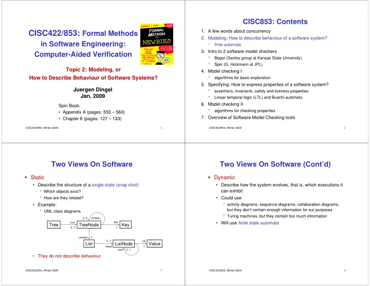
Two Views On Software

Static

• Describe the structure of a single state (snap shot)

° Which objects exist? ° How are they related?

• Example:

° UML class diagrams

• They do not describe behaviour

Tree TreeNode List Key

0..2 0..1 root children content key 1 1

ListNode

head 0..1 next 0..1

Value

val 1 CISC422/853, Winter 2009 4

Two Views On Software (Cont’d)

Dynamic

• Describe how the system evolves, that is, which executions it

can exhibit

• Could use

° activity diagrams, sequence diagrams, collaboration diagrams, but they don’t contain enough information for our purposes ° Turing machines, but they contain too much information

• Will use finite state automata

CISC422/853, Winter 2009 5

Finite State Automaton

A finite state automaton (machine) is a tuple (S, S0, L, δ, F) where S is a finite set of states S0 is a set of distinguished initial states with S0⊆ S L is a finite set of labels δ is a set of transitions with δ⊆(S×L×S) F is a set of final states with F⊆S A finite state automaton (machine) is a tuple (S, S0, L, δ, F) where S is a finite set of states S0 is a set of distinguished initial states with S0⊆ S L is a finite set of labels δ is a set of transitions with δ⊆(S×L×S) F is a set of final states with F⊆S

s0 s1 s2 s3 s4 Example: l0 l0 l1 l2

CISC422/853, Winter 2009 6

Transitions

System makes one step from one state to another Transitions can be enabled ...

• transition (si, l, si+1) is enabled in state si,iff (si, l, si+1) ∈ δ

... or disabled

• transition (si, l, si+1) is disabled in state si iff (si, l, si+1)∉δ

Transition labels can contain information about, e.g.,

• which process is carrying out the transition
• how much time the transition is taking (Timed automata)
• how likely it is that the transition is taken (probabilistic

automata, Markov processes)

• an instruction (e.g., guard, assignment, input, output)

s0 s2 s1 stop start

CISC422/853, Winter 2009 7

Non-determinism

Non-determinism is useful to

• model concurrent computations

° to abstract from particular scheduling policies

• model incompletely specified inputs or environments

° to abstract from particular inputs or environments

• write test harnesses

An FSA (S, S0, L, δ, F) is deterministic iff ∀ s,s1,s2∈S. ∀ l∈L. (s, l, s1)∈δ Æ (s, l, s2)∈δ ⇒ s1=s2 An FSA is non-deterministic iff it’s not deterministic. An FSA (S, S0, L, δ, F) is deterministic iff ∀ s,s1,s2∈S. ∀ l∈L. (s, l, s1)∈δ Æ (s, l, s2)∈δ ⇒ s1=s2 An FSA is non-deterministic iff it’s not deterministic.

CISC422/853, Winter 2009 8

Runs and (Standard) Acceptance

A run (a.k.a., execution, trace) σ of an FSA (S, S0, L, δ, F) is a possibly infinite sequence of transitions (s0, l0, s1)(s1, l1, s2)(s2, l2, s3)… such that ∀0≤ i<|σ|. (si, li, si+1)∈δ. An ω-run is an infinite run. A run (a.k.a., execution, trace) σ of an FSA (S, S0, L, δ, F) is a possibly infinite sequence of transitions (s0, l0, s1)(s1, l1, s2)(s2, l2, s3)… such that ∀0≤ i<|σ|. (si, li, si+1)∈δ. An ω-run is an infinite run. A accepting run of an FSA (S, S0, L, δ, F) is a finite run (s0, l0, s1)(s1, l1, s2)(s2, l2, s3)…(sn-1, ln−1,sn) such that s0∈S0 and sn∈F. A accepting run of an FSA (S, S0, L, δ, F) is a finite run (s0, l0, s1)(s1, l1, s2)(s2, l2, s3)…(sn-1, ln−1,sn) such that s0∈S0 and sn∈F.

“An accepting run is a run that ends in a final state”

At this point, accepting runs are always finite!

CISC422/853, Winter 2009 9

Reachable States

The reachable states (a.k.a., state space) of an FSA A is the set of all states along every run of A from an initial state. The reachable states (a.k.a., state space) of an FSA A is the set of all states along every run of A from an initial state.

s0 s1 s2 s3 s4 Example: l0 l0 l1 l2 has reachable states {s0, s1, s2, s3} The FSA “All states s to which there is a path from s0 ∈ S0 to s”

CISC422/853, Winter 2009 10

Words and Languages

The language L(A) of an FSA A is the set of words of A: L(A) = { w | w is word of A} The language L(A) of an FSA A is the set of words of A: L(A) = { w | w is word of A} A word w of an FSA A is the sequence of labels l0l1l2 … ln of an accepting run (s0, l0, s1)(s1, l1, s2)(s2, l2, s3)…(sn-1, ln−1,sn)

• f A.

A word w of an FSA A is the sequence of labels l0l1l2 … ln of an accepting run (s0, l0, s1)(s1, l1, s2)(s2, l2, s3)…(sn-1, ln−1,sn)

• f A.

Example: A1=

L(A1) = start run ((pre-empt run)* (block unblock)*)* stop

Theorem: FSAs = regular expressions = regular languages

CISC422/853, Winter 2009 11

Asynchronous Composition

The asynchronous composition of 2 FSAs A and B is an FSA A||B such that A||B = (S, S0, L, δ, F) where S is the Cartesian product A.S × B.S S0 is { (a0, b0)∈S | a0∈ A.S0 Æ b0∈ B.S0} L is the union A.L ∪ B.L δ is {((a1, b), l, (a2, b))∈S×L×S | (a1,l,a2)∈ A.δ} ∪ {((a, b1), l, (a, b2))∈S×L×S | (b1,l,b2)∈ B.δ} F is {(s1, s2) ∈ S | s1∈A.F Ç s2∈B.F} The asynchronous composition of 2 FSAs A and B is an FSA A||B such that A||B = (S, S0, L, δ, F) where S is the Cartesian product A.S × B.S S0 is { (a0, b0)∈S | a0∈ A.S0 Æ b0∈ B.S0} L is the union A.L ∪ B.L δ is {((a1, b), l, (a2, b))∈S×L×S | (a1,l,a2)∈ A.δ} ∪ {((a, b1), l, (a, b2))∈S×L×S | (b1,l,b2)∈ B.δ} F is {(s1, s2) ∈ S | s1∈A.F Ç s2∈B.F}

where A.S denotes the set of states of FSA A etc

Æ would result In a stronger acceptance condition

CISC422/853, Winter 2009 12

Example: Asynchronous Composition (1)

s0 s1

eat drink

t0 t1

dance sing

A B (s0,t0) (s1,t0) (s0,t1) (s1,t1) A || B

dance sing dance sing eat drink eat drink

CISC422/853, Winter 2009 13

Example: Asynchronous Composition (2)

t1

x%2!=0Æx>1? x:=3x+1

t0 A || B (s0,t0) (s1,t0) (s0,t1) (s1,t1)

x:=3x+1

x%2!=0Æx>1? x%2!=0Æx<1?

x%2=0? x:=x/2 x%2=0? x:=x/2 x:=3x+1

(s2,t0)

x=1

(s2,t1)

x=1

s0 s1

x%2=0? x:=x/2

s2

x=1?

A B

CISC422/853, Winter 2009 14

Asynchronous Composition (Cont’d)

Form of parallel composition that allows each process to move completely independently of other processes Models our intuition about parallel or distributed processes executing at different speeds Introduces possibility of unfair executions, that is, executions in which, after some finite amount time, a process not executed anymore (e.g., P1 P2 P1 P2 P1 P1 P1 … )

• Only infinite executions can be unfair (more on fairness later)

Related concepts:

• asynchronous communication:

° process can send w/o having to block until a matching receive is executed

qE.g., communication channel is implemented as a buffer

° Examples: Unix sockets, email

• asynchronous circuits

CISC422/853, Winter 2009 15

Synchronous Composition

The synchronous composition of 2 FSAs A and B is an FSA A⊗B such that A⊗B = (S, S0, L, δ, F) where S is A.S × B.S S0 is { (a0, b0)∈S | a0 ∈ A.S0 Æ b0 ∈ B.S0} L is A.L × B.L δ is {((s,t), (l1,l2), (s’,t’))∈ S×L×S | (s, l1, s’)∈A.δ Æ (t, l2, t’)∈B.δ} F is {(s1, s2) ∈ S | s1∈A.F Ç s2∈B.F} The synchronous composition of 2 FSAs A and B is an FSA A⊗B such that A⊗B = (S, S0, L, δ, F) where S is A.S × B.S S0 is { (a0, b0)∈S | a0 ∈ A.S0 Æ b0 ∈ B.S0} L is A.L × B.L δ is {((s,t), (l1,l2), (s’,t’))∈ S×L×S | (s, l1, s’)∈A.δ Æ (t, l2, t’)∈B.δ} F is {(s1, s2) ∈ S | s1∈A.F Ç s2∈B.F}

CISC422/853, Winter 2009 16

Example: Synchronous Composition

!(x%2)

t0 t1

• ne

A B A ⊗ B

drink

t2

two

t3

viol viol

x=3x+1 !(x%2)

s0t0 s0t1

(drink,one)

B

s0t2

(drink,two)

S0t3

(drink,viol) (drink,viol)

s0

CISC422/853, Winter 2009 17

Synchronous Composition (Cont’d)

Form of parallel composition in which all processes have to move in lockstep Models our intuition about the execution of processes being controlled by a global clock Related concepts:

• synchronous communication:

° process executing a send blocks until receiving process executes a matching receive qE.g., communication buffer is filled to capacity ° Examples: telephone, rendezvous

• synchronous circuits

CISC422/853, Winter 2009 18

Useful for “monitoring”, that is, the continuous

• bservation (and checking) of one process by another

Later, we will see how a property ϕ can be expressed with an automaton Aϕ Then, Aϕ is the monitor process For example, B (from before) is monitor process for “# of ‘drinks > 2”

Synchronous Composition (Cont’d)

x=x/2 !(x%2)

Observation:

For any process P, P⊗Aϕ has an accepting run iff P can satisfy ϕ iff P can violate ¬ϕ

Observation:

For any process P, P⊗Aϕ has an accepting run iff P can satisfy ϕ iff P can violate ¬ϕ

CISC422/853, Winter 2009 19

Previously,

• states and labels could be anything

Now,

• states: uniquely describes particular “snapshot” during execution

° values of all global variables in S, and ° for all threads t,

qvalue of program counter of t, and qvalues of local variables of t

• labels: may describe how to get from one state to the next

° statements (e.g., “y:=0;x:=x+y”), or ° guards (e.g., “x≥ 4”, “x even”)

• rest (i.e., initial and final states and transition relation): as before

Interpreted FSAs (iFSAs)

State may have to contain more info, but for us, this suffices

CISC422/853, Winter 2009 20

Formally, A = (S, S0, L, δ, F) where

S = {(sP,sV) | sP∈PC→Loc Æ sV∈Vars→D} where

Vars = set of variables D = set of values PC = set of program counters Loc = set of locations Notation: A.V = Vars // all variables used/defined in A A.P = PC // all program counters used/defined in A

L ::= <stmt> | <guard>? where

<stmt> ::= <var>:=<exp> | <stmt>;<stmt> | … <var> ∈ Var

// variable used in labels is assigned value // in states, i.e., varsUsedIn(A.L) ⊆ A.V = Vars

<exp> is “expression over variables in A.V” <guard> ::= <exp><relop><exp> | <guard> <boolop> <guard>

all finite

Interpreted FSAs (iFSAs) (Cont’d)

A different/ richer language for L is possible here A different/ richer language for L is possible here L sometimes also called “Action Language” L sometimes also called “Action Language”

CISC422/853, Winter 2009 21

Interpreted FSAs (iFSAs) (Cont’d)

• But, now need to make sure that
• 1. Labels are consistent with states:

Definition of (s,l,t)∈δ can’t ignore label l anymore

An interpreted finite state automaton (machine) is a tuple (S, S0, L, δ, F) where S … // as on previous slide S0 ⊆ S // as before

δ

is {((sP,sV),l,(tP,tV)) ∈ S×L×S | (sV,tV) is consistent with l} where

(sV,tV) consistent w/ stmt p iff “execution of p from state sV terminates in state tV” (sV,tV) consistent w/ guard b iff “b evaluates to ‘true’ in sV” and sV = tV

F ⊆ S // as before An interpreted finite state automaton (machine) is a tuple (S, S0, L, δ, F) where S … // as on previous slide S0 ⊆ S // as before

δ

is {((sP,sV),l,(tP,tV)) ∈ S×L×S | (sV,tV) is consistent with l} where

(sV,tV) consistent w/ stmt p iff “execution of p from state sV terminates in state tV” (sV,tV) consistent w/ guard b iff “b evaluates to ‘true’ in sV” and sV = tV

F ⊆ S // as before

CISC422/853, Winter 2009 22

Interpreted FSAs (iFSAs) (Cont’d)

Example: iFSA for 3n+1 problem with x=8 initially

[pc=0,x=8] [pc=1,x=8] [pc=1,x=4] [pc=0,x=4] [pc=0,x=2] [pc=1,x=2]

x:=x/2 x:=x/2 x%2=0?

[pc=0,x=1] [pc=2,x=1] x%2=0?

x%2=0? x:=x/2 x=1?

CISC422/853, Winter 2009 23

Translating FSAs into iFSAs

Let

• FSA A = (S, S0, L, δ, F)

// L is some standard action language

• Vars = varsIn(A.L)

// variables used in labels in A

• D some finite domain // e.g., D = {i ∈ ℕ| i ≤ 100}

We can compute the corresponding iFSA intVars,D(A) = (S’, S’0, L, δ’, F’) where

S’ = intVars,D(S) S’0 = intVars,D(S0) δ’ = {((pcA=s, sV), l, (pcA=t, tV)) | (s, l, t) ∈ δ Æ sV∈ Vars→ D Æ tV∈ Vars→ D Æ (sV, tV) consistent with l} F’ = intVars,D(F) where intVars,D(S) = {(pcA=s, sV) | s∈S Æ sV∈ Vars→D}

CISC422/853, Winter 2009 24

Translating FSAs into iFSAs (Cont’d)

Example 1:

s0 s1 s2 x<2? x:=x+1 x≥2?

A intVars,D(A) Let D = {0, 1, 2, 3, 4} and Vars = {x}

[0,0] [1,0] [0,1] [1,1] [0,2] [2,2] [0,3] [2,3] [0,4] [2,4]

[i,j] abbreviates [pcA=si, x=j]

x:=x+1 x:=x+1 x<2? x<2? x≥2? x≥2? x≥2?

CISC422/853, Winter 2009 25

Translating FSAs into iFSAs (Cont’d)

Example 2:

intVars,D(A) where Vars = {x} and D = {n ∈ ℕ | n ≤16} s0 s1

x%2=0? x:=x/2

s2

x=1?

A

[i,j] abbreviates [pcA=si, x=j]

[0,16] [0,15] [0,14] [0,13] [0,12] [0,11] [0,10] [0,9] [0,8] [0,7] [0,6] [0,5] [0,4] [0,3] [0,2] [0,1] [0,0] [1,16] [1,14] [1,12] [1,10] [1,8] [1,6] [1,4] [1,2] [2,1] x=1?

x%2=0?

x:=x/2

CISC422/853, Winter 2009 26

The asynchronous composition of 2 FSAs A and B is an FSA A||B such that A||B = (S, s0, L, δ, F) where S is {((sP,sV), (tP,tV)) ∈ A.S×B.S | sV, tV don’t conflict} … // unchanged The asynchronous composition of 2 FSAs A and B is an FSA A||B such that A||B = (S, s0, L, δ, F) where S is {((sP,sV), (tP,tV)) ∈ A.S×B.S | sV, tV don’t conflict} … // unchanged

Interpreted FSAs (iFSAs) (Cont’d)

Need to make sure that

2) Composition operations result in consistent states:

“In state (s,t), variable assignment of s must not conflict with that of t”

where sV, tV don’t conflict iff

• ∀x∈(A.VÅB.V) . sV(x) = tV(x) and

// A and B agree on shared vars

• A.PÅB.P = ∅

// A and B use different program counters

CISC422/853, Winter 2009 27

Interpreted FSAs (iFSAs) (Cont’d)

Need to make sure that

2) Composition operations result in consistent states:

“In state (s,t), variable assignment of s must not conflict with that of t”

where sV, tV don’t conflict iff

• ∀x∈(A.VÅB.V) . sV(x) = tV(x) and
• A.PÅB.P = ∅

The synchronous composition of 2 FSAs A and B is an FSA A⊗B such that A⊗B = (S, s0, L, δ, F) where S is {((sP,sV), (tP,tV)) ∈ A.S×B.S | sV, tV don’t conflict} … // unchanged The synchronous composition of 2 FSAs A and B is an FSA A⊗B such that A⊗B = (S, s0, L, δ, F) where S is {((sP,sV), (tP,tV)) ∈ A.S×B.S | sV, tV don’t conflict} … // unchanged

CISC422/853, Winter 2009 28

Interpreted FSAs (iFSAs) (Cont’d)

Example 1: 3n+1 w/ full variable info

s0 s1

x%2=0? x:=x/2

s2

x=1?

A t1

x%2!=0Æx>1? x:=3x+1

t0 B intVars,D(A) || intVars,D(B) where Vars={x} and D = {0, …, 16}

[i,j,k] abbreviates [pcA=si, pcB=tj, x=k]

[0,0,16] [0,0,15] [0,0,14] [0,0,13] [0,0,12] [0,0,11] [0,0,10] [0,0,9] [0,0,8] [0,0,7] [0,0,6] [0,0,5] [0,0,4] [0,0,3] [0,0,2] [0,0,1] [0,0,0] [1,0,16] [1,0,14] [1,0,12] [1,0,10] [1,0,8] [1,0,6] [1,0,4] [1,0,2] [2,0,1] [0,1,5] [0,1,3] [0,1,15] [0,1,13] [0,1,11] [0,1,9] [0,1,7]

labels are elided

CISC422/853, Winter 2009 29

Interpreted FSAs (iFSAs) (Cont’d)

Example 2: 3n+1 w/ full variable info w/ monitor C

u1 u0 C

x<3?

(intVars,D(A) || intVars,D(B)) ⊗ intVars,D(C)

where Vars={x} and D = {0, …, 16}

true? x<3?

and [i,j,k,l] abbreviates [pcA=si,pcB=tj,pcC=uk,x=l] where

[0,0,0,6] [0,0,0,5] [0,0,0,4] [0,0,0,3] [0,0,0,2] [0,0,0,1] [0,0,0,0] [1,0,0,6] [1,0,0,4] [1,0,0,2] [2,0,1,1] [0,1,0,5] [0,1,0,3] [1,0,1,2] [0,0,1,1]

a1?,c1 a1?,c1 a1?,c1 a1?,c1 a1?,c1 a2,c1 a2,c1 a2,c1 a1?,c2? a2,c2? a2,c2? a3?,c2?

[2,0,0,1]

a3?,c1 a3?,c2? a1 ≡ x%2=0, a2 ≡ x:=x/2, a3 ≡ x=1, c1 ≡ true, c2 ≡ x<3 Note non- determinism in C Note non- determinism in C

CISC422/853, Winter 2009 30

FSAs and iFSAs: Notes

Note

• Typically, FSA used for representation, but
• analysis always done on iFSA

Given FSA A, corresponding iFSA int(A) computed either

• before analysis
• during analysis (on the fly)

° This is what the “Semantics Engine” in the Spin Textbook does [Hol04, Chapter 7]

CISC422/853, Winter 2009 31

FSAs: Extensions

Another notational abbreviation: Composite (hierarchical) states

• With sequential substates: E.g.,

which abbreviates

init read process write error

failure failure failure failure

init read process write error

failure

These kinds

• f composite

states are also known as “or-states” (b/c at most

• ne of the

immediate substates is active) These kinds

• f composite

states are also known as “or-states” (b/c at most

• ne of the

immediate substates is active)

CISC422/853, Winter 2009 32

FSAs: Extensions (Cont’d)

Another notational abbreviation: Composite (hierarchical) states

• With sequential substates
• With concurrent substates (orthogonal regions)

s0 s1 t0 t1

These kinds

• f composite

states are also known as “and-states” (b/c, all immediate Substates are active) These kinds

• f composite

states are also known as “and-states” (b/c, all immediate Substates are active)

CISC422/853, Winter 2009 33

FSAs: Extensions (Cont’d)

Another notational abbreviation: Composite (hierarchical) states w/ sequential & concurrent substates Transition labeled with trigger t, guard g and action a History states

t[g]/a

init read process write error

failure

fix

H

UML State Machines and StateCharts [Harel 1984] have all of these extensions UML State Machines and StateCharts [Harel 1984] have all of these extensions

CISC422/853, Winter 2009 34

Example: StateCharts

• F. Stolzenburg. From the Specification of Multiagent Systems by Statecharts to their

Formal Analysis by Model Checking. Fachberichte INFORMATIK. Universitaet Koblenz, Germany. June 2001.

CISC422/853, Winter 2009 35

Alternatives to FSAs

Process algebras:

• Calculus of Communicating Systems (CCS) [Milner, 1980]
• Communicating Sequential Processes (CSP) [Hoare, 1985]
• Lotos (Language of Temporal Ordering Specifications) [1989]
• Estelle [1986]

Petri nets [Petri, 1960]

CISC422/853, Winter 2009 36

Example: CCS

• Let

C ≡ coin.coffee.C // coffee machine P ≡ coin.coffee.publish.P // professor

• The (synchronous) parallel composition of C and P is

P | C ≡ coin.coffee.publish.P | coin.coffee.C

• Using the equational laws of CCS we can deduce that P | C is an

infinite publishing machine: P | C = τ.τ.publish.(P | C) = publish.(P | C)

• CCS neatly captures basic notions of concurrency, e.g.,
• communication, synchronization, input, output, observability

and the rules that govern it, e.g.,

• P | Q = Q | P
• a.P | a.Q = τ.(P | Q) = P | Q
• a.P | b.Q = a.(P | b.Q) + b.(a.P | Q)

CISC422/853, Winter 2009 37

Example: Petri Nets

transition place token/ marking enabled transition

http://www.informatik.uni-hamburg.de/TGI/PetriNets/introductions/aalst/ CISC422/853, Winter 2009 38

Simple Petri Nets

A Simple Petri Net is a tuple N = (P, M0, T, pre, post, MF) where P is a finite set of places M0 ⊆ P is the initial marking T is a finite set of transitions pre: T→ 2P defines the pre-set of each transition post: T→ 2P defines the post-set of each transition MF ⊆ P is the final marking // a bit non-standard A Simple Petri Net is a tuple N = (P, M0, T, pre, post, MF) where P is a finite set of places M0 ⊆ P is the initial marking T is a finite set of transitions pre: T→ 2P defines the pre-set of each transition post: T→ 2P defines the post-set of each transition MF ⊆ P is the final marking // a bit non-standard

CISC422/853, Winter 2009 39

Simple Petri Nets (Cont’d)

Let N = (P, M0, T, pre, post, MF) and t be a transition in N (i.e., t∈T) and M be a marking in N (i.e., M ⊆ P) We say t is enabled in M iff pre(t) ⊆ M If t enabled in M, then firing t in M creates new marking M’ = (M\pre(t)) ∪ post(t) Execution of N consists of repeated firings of enabled transitions from initial marking until final marking is reached Let N = (P, M0, T, pre, post, MF) and t be a transition in N (i.e., t∈T) and M be a marking in N (i.e., M ⊆ P) We say t is enabled in M iff pre(t) ⊆ M If t enabled in M, then firing t in M creates new marking M’ = (M\pre(t)) ∪ post(t) Execution of N consists of repeated firings of enabled transitions from initial marking until final marking is reached So, simple Petri nets seem similar to FSAs…

CISC422/853, Winter 2009 40

Simple Petri Nets as FSAs

Let N = (P, M0, T, pre, post, MF). Corresponding FSAN is given by (S, S0, L, δ, F) where S = 2P S0 = {M0} ⊆ S L = T δ = {(M, t, M’) ∈ S×L×S | pre(t)⊆M Æ M’=(M\pre(t)) ∪ post(t)} F = {MF} ⊆ S Let N = (P, M0, T, pre, post, MF). Corresponding FSAN is given by (S, S0, L, δ, F) where S = 2P S0 = {M0} ⊆ S L = T δ = {(M, t, M’) ∈ S×L×S | pre(t)⊆M Æ M’=(M\pre(t)) ∪ post(t)} F = {MF} ⊆ S

⇒ One-to-one correspondence between accepting runs in FSAN and executions in simple Petri net N Caveat: There is a whole lot more to Petri nets than what we’ve discussed here…

CISC422/853, Winter 2009 41

Modeling Behaviour of Systems

Where are we?

• We’ve decided to use FSAs to model the behaviour of

software systems

• Have seen:

° Two types of parallel composition ° Uninterpreted vs interpreted ° Extensions ° Some of the alternatives (e.g., Process algebra, Petri nets)

What’s next?

• But, to be able to feed FSAs into a model checker, we need to

be able to express FSAs textually in some language

• Also, it would be nice if that language was as high-level (user-

friendly) as possible.

• 2 examples for modeling languages based on FSAs:

° BIR (used by Bogor model checker) ° Promela (used by Spin model checker)