Find the inverse Z-transform of 2 z 2 + 2 z G ( z ) = z 2 + 2 z 3 G - - PowerPoint PPT Presentation

1.

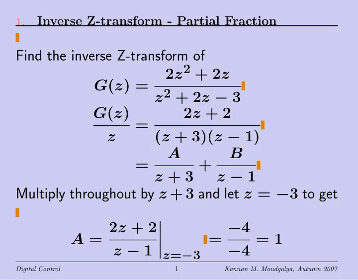
Inverse Z-transform - Partial Fraction

Find the inverse Z-transform of G(z) = 2z2 + 2z z2 + 2z − 3 G(z) z = 2z + 2 (z + 3)(z − 1) = A z + 3 + B z − 1 Multiply throughout by z +3 and let z = −3 to get A = 2z + 2 z − 1

• z=−3

= −4 −4 = 1

Digital Control

1

Kannan M. Moudgalya, Autumn 2007

2.

Inverse Z-transform - Partial Fraction

G(z) z = A z + 3 + B z − 1 Multiply throughout by z − 1 and let z = 1 to get B = 4 4 = 1 G(z) z = 1 z + 3 + 1 z − 1 |z| > 3 G(z) = z z + 3 + z z − 1 |z| > 3 ↔ (−3)n1(n) + 1(n)

Digital Control

2

Kannan M. Moudgalya, Autumn 2007

3.

Partial Fraction - Repeated Poles G(z) = N(z) (z − α)pD1(z) α not a root of N(z) and D1(z) G(z) = A1 z − α + A2 (z − α)2 + · · · + Ap (z − α)p + G1(z) G1(z) has poles corresponding to those of D1(z). Multiply by (z − α)p (z − α)pG(z) = A1(z − α)p−1 + A2(z − α)p−2 + · · · + Ap−1(z − α) + Ap + G1(z)(z − α)p

Digital Control

3

Kannan M. Moudgalya, Autumn 2007

4.

Partial Fraction - Repeated Poles (z − α)pG(z) = A1(z − α)p−1 + A2(z − α)p−2 + · · · + Ap−1(z − α) + Ap + G1(z)(z − α)p Substituting z = α, Ap = (z − α)pG(z)|z=α Differentiate and let z = α: Ap−1 = d dz(z − α)pG(z)|z=α Continuing, A1 = 1 (p − 1)! dp−1 dzp−1(z − α)pG(z)|z=α

Digital Control

4

Kannan M. Moudgalya, Autumn 2007

5.

Repeated Poles - an Example G(z) = 11z2 − 15z + 6 (z − 2)(z − 1)2 = A1 z − 1 + A2 (z − 1)2 + B z − 2 × (z − 2), let z = 2, to get B = 20. × (z − 1)2, 11z2 − 15z + 6 z − 2 = A1(z − 1) + A2 + B(z − 1)2 z − 2 With z = 1, get A2 = −2. Differentiating with respect to z and with z = 1, A1 = (z − 2)(22z − 15) − (11z2 − 15z + 6) (z − 2)2

• z=1

= −9 G(z) = − 9 z − 1 − 2 (z − 1)2 + 20 z − 2

Digital Control

5

Kannan M. Moudgalya, Autumn 2007

6.

Important Result from Differentiation Problem 4.9 in Text: Consider 1(n)an ↔ z z − a =

∞

• n=0

anz−n,

• az−1

< 1 Differentiating with respect to a, z (z − a)2 =

∞

• n=0

nan−1z−n, nan−11(n) ↔ z (z − a)2 Substituting a = 1, can obtain the Z-transform of n: n1(n) ↔ z (z − 1)2 Through further differentiation, can derive Z-transforms of n2, n3, etc.

Digital Control

6

Kannan M. Moudgalya, Autumn 2007

7.

Repeated Poles - an Example

G(z) = − 9 z − 1 − 2 (z − 1)2 + 20 z − 2 zG(z) = − 9z z − 1 − 2z (z − 1)2 + 20z z − 2 ↔ (−9 − 2n + 20 × 2n)1(n) Use shifting theorem:

G(z) ↔ (−9 − 2(n − 1) + 20 × 2n−1)1(n − 1)

Digital Control

7

Kannan M. Moudgalya, Autumn 2007

8.

Properties of Cont. Time Sinusoidal Signals

ua(t) = A cos (Ωt + θ) ua(t) = A cos (2πF t + θ), − ∞ < t < ∞ A: amplitude Ω: frequency in rad/s θ: phase in rad F : frequency in cycles/s or Hertz Ω = 2πF Tp = 1 F

Digital Control

8

Kannan M. Moudgalya, Autumn 2007

9.

Properties of Cont. Time Sinusoidal Signals

ua(t) = A cos (Ωt + θ) ua(t) = A cos (2πF t + θ), − ∞ < t < ∞ With F fixed, periodic with period Tp ua[t + Tp] = A cos (2πF (t + 1 F ) + θ) = A cos (2π + 2πF t + θ) = A cos (2πF t + θ) = ua[t]

Digital Control

9

Kannan M. Moudgalya, Autumn 2007

10.

Properties of Cont. Time Sinusoidal Signals

• Cont. signals with different frequencies are different

u1 = cos

• 2π t

8

• , u2 = cos
• 2π7t

8

• 0.5

1 1.5 2 2.5 3 3.5 4 −1 −0.8 −0.6 −0.4 −0.2 0.2 0.4 0.6 0.8 1 t coswt

Different wave forms for different frequencies. Can increase f all the way to ∞ or decrease to 0.

Digital Control

10

Kannan M. Moudgalya, Autumn 2007

11.

Discrete Time Sinusoidal Signals

u(n) = A cos (wn + θ), −∞ < n < ∞ w = 2πf n integer variable, sample number A amplitude of the sinusoid w frequency in radians per sample θ phase in radians. f normalized frequency, cycles/sample

Digital Control

11

Kannan M. Moudgalya, Autumn 2007

12.

Discrete Time Sinusoids - Identical Signals

Discrete time sinusoids whose frequencies are sepa- rated by integer multiple of 2π are identical, i.e., cos ((w0 + 2π)n + θ) = cos (w0n + θ), ∀n

• All sinusoidal sequences of the form,

uk(n) = A cos (wkn + θ), wk = w0 + 2kπ, −π < w0 < π, are indistinguishable or identical.

• Only sinusoids in −π < w0 < π are different

−π < w0 < π or − 1 2 < f0 < 1 2

Digital Control

12

Kannan M. Moudgalya, Autumn 2007

13.

Sampling a Cont. Time Signal - Preliminaries

Let analog signal ua[t] have a frequency of F Hz ua[t] = A cos(2πF t + θ) Uniform sampling rate (Ts s) or frequency (Fs Hz) t = nTs = n Fs u(n) = ua[nTs] − ∞ < n < ∞ = A cos (2πF Tsn + θ) = A cos

• 2π F

Fs n + θ

• △

= A cos(2πfn + θ)

Digital Control

13

Kannan M. Moudgalya, Autumn 2007

14.

Sampling a Cont. Time Signal - Preliminaries

In our standard notation, u(n) = A cos (2πfn + θ) It follows that f = F Fs w = Ω Fs = ΩTs Reason to call f normalized frequency, cycles/sample. Apply the uniqueness condition for sampled signals − 1 2 < f < 1 2 −π < w < π Fmax = Fs 2 Ωmax = 2πFmax = πFs = π Ts

Digital Control

14

Kannan M. Moudgalya, Autumn 2007

15.

Properties of Discrete Time Sinusoids - Alias

• As w0 ↑, freq. of oscillation ↑, reaches maximum

at w0 = π

• What if w0 > π?

w1 = w0 w2 = 2π − w0 u1(n) = A cos w1n = A cos w0n u2(n) = A cos w2n = A cos(2π − w0)n = A cos w0n = u1(n) w2 is an alias of w1

Digital Control

15

Kannan M. Moudgalya, Autumn 2007

16.

Properties of Discrete Time Sinusoids - Alias u1[t] = cos (2π t 8), u2[t] = cos (2π7t 8 ), Ts = 1 u2(n) = cos (2π7n 8 ) = cos 2π(1 − 1 8)n = cos (2π − 2π 8 )n = cos (2πn 8 ) = u1(n)

0.5 1 1.5 2 2.5 3 3.5 4 −1 −0.8 −0.6 −0.4 −0.2 0.2 0.4 0.6 0.8 1

t coswt

Digital Control

16

Kannan M. Moudgalya, Autumn 2007

17.

Fourier Transform of Aperiodic Signals

X(F ) = ∞

−∞

x(t)e−j2πF tdt x(t) = ∞

−∞

X(F )ej2πF tdF If we let radian frequency Ω = 2πF x(t) = 1 2π ∞

−∞

X[Ω]ejΩtdΩ, X[Ω] = ∞

−∞

x(t)e−jΩtdt x(t), X[Ω] are Fourier Transform Pair

Digital Control

17

Kannan M. Moudgalya, Autumn 2007

18.

Frequency Response Apply u(n) = ejwn to g(n) and obtain output y: y(n) = g(n) ∗ u(n) =

∞

• k=−∞

g(k)u(n − k) =

∞

• k=−∞

g(k)ejw(n−k) = ejwn

∞

• k=−∞

g(k)e−jwk Define Discrete Time Fourier Transform G(ejw)

△

=

∞

• k=−∞

g(k)e−jwk =

∞

• k=−∞

g(k)z−k

• z=ejw

= G(z)|z=ejw Provided the sequence converges absolutely

Digital Control

18

Kannan M. Moudgalya, Autumn 2007

19.

Frequency Response y(n) = ejwn

∞

• k=−∞

g(k)e−jwk = ejwnG(ejw) Write in polar coordinates: G(ejw) = |G(ejw)|ejϕ - ϕ is phase angle: y(n) = ejwn|G(ejw)|ejϕ = |G(ejwn)|ej(wn+ϕ)

• 1. Input is sinusoid ⇒ output also is a sinusoid with following

properties:

• Output amplitude gets multiplied by the magnitude of

G(ejw)

• Output sinusoid shifts by ϕ with respect to input

Digital Control

19

Kannan M. Moudgalya, Autumn 2007

• 2. At ω where |G(ejw)| is large, the sinusoid gets amplified

and at ω where it is small, the sinusoid gets attenuated.

• The system with large gains at low frequencies and small

gains at high frequencies are called low pass filters

• Similarly high pass filters

Digital Control

20

Kannan M. Moudgalya, Autumn 2007

20.

Discrete Fourier Transform Define Discrete Time Fourier Transform G(ejw)

△

=

∞

• k=−∞

g(k)e−jwk =

∞

• k=−∞

g(k)z−k

• z=ejw

= G(z)|z=ejw Provided, absolute convergence

∞

• k=−∞

|g(k)e−jwk| < ∞ ⇒

∞

• k=−∞

|g(k)| < ∞ For causal systems, BIBO stability. Required for DTFT.

Digital Control

21

Kannan M. Moudgalya, Autumn 2007

21.

FT of Discrete Time Aperiodic Signals - Defi- nition U(ejω)

△

=

∞

• n=−∞

u(n)e−jωn u(m) = 1 2π π

−π

U(ejω)ejωmdω = 1/2

−1/2

U(f)ej2πfmd f

Digital Control

22

Kannan M. Moudgalya, Autumn 2007

22.

FT of a Moving Average Filter - Example y(n) = 1 3[u(n + 1) + u(n) + u(n − 1)] y(n) =

∞

• k=−∞

g(k)u(n − k) = g(−1)u(n + 1) + g(0)u(n) + g(1)u(n − 1) g(−1) = g(0) = g(1) = 1 3 G

• ejw

=

∞

• n=−∞

g(n)z−n|z=ejw = 1 3

• ejw + 1 + e−jw

= 1 3(1 + 2 cos w)

Digital Control

23

Kannan M. Moudgalya, Autumn 2007

23.

FT of a Moving Average Filter - Example G

• ejω

= 1 3(1 + 2 cos w), |G

• ejw

| = |1 3(1 + 2 cos w)| Arg(G) =

• 0 ≤ w < 2π

3

π

2π 3 ≤ w < π

1

/ / U p d a t e d ( 1 8 − 7 − 0 7 )

2

/ / 5 . 3

3 4 w = 0 : 0 . 0 1 : %pi ; 5 subplot (2 ,1 ,1); 6 plot2d1 (” g l l ” ,w, abs(1+2∗cos (w))/3 , s t y l e = 2); 7 l a b e l ( ’ ’ ,4 , ’

’ , ’ Magnitude ’ ,4);

8 subplot (2 ,1 ,2); 9 plot2d1 (” gln ” ,w, phasemag(1+2∗cos (w)) , s t y l e = 2 , r e c t

=[0.

10 l a b e l ( ’ ’ ,4 , ’w ’ , ’ Phase ’ ,4)

Digital Control

24

Kannan M. Moudgalya, Autumn 2007

24.

FT of a Moving Average Filter - Example |G

• ejw

| = |1 3(1 + 2 cos w)|, Arg(G) =

• 0 ≤ w < 2π

3

π

2π 3 ≤ w < π

10

−2

10

−1

10 10

1

10

−3

10

−2

10

−1

10

Magnitude

10

−2

10

−1

10 10

1

50 100 150 200

w Phase

Digital Control

25

Kannan M. Moudgalya, Autumn 2007

25.

Additional Properties of Fourier Transform Symmetry of real and imaginary parts for real valued sequences G

• ejw

=

∞

• n=−∞

g(n)e−jwn =

∞

• n=−∞

g(n) cos wn − j

∞

• n=−∞

g(n) sin wn G

• e−jw

=

∞

• n=−∞

g(n)ejwn =

∞

• n=−∞

g(n) cos wn + j

∞

• n=−∞

g(n) sin wn Re

• G
• ejw

= Re

• G
• e−jw

Im

• G
• ejw

= −Im

• G
• e−jw

Digital Control

26

Kannan M. Moudgalya, Autumn 2007

26.

Additional Properties of Fourier Transform Recall G

• ejw

= G∗ e−jw Symmetry of magnitude for real valued sequences |G

• ejw

| =

• G
• ejw

G∗ ejw1/2 =

• G∗

e−jw G

• e−jw1/2

= |G(e−jw)| This shows that the magnitude is an even function. Similarly, Arg

• G
• e−jw

= −Arg

• G
• ejw

⇒ Bode plots have to be drawn for w in [0, π] only.

Digital Control

27

Kannan M. Moudgalya, Autumn 2007

27.

Sampling and Reconstruction u(n) = ua(nTs), −∞ < n < ∞ Fast sampling:

Fs 2

Ts F t −B

B

−Fs

2

−3

2Fs 3 2Fs

Ua(F ) ua(nT ) = u(n) U

• F

Fs

• 1

Fs ua(t) t F

Fs 2

F0 + Fs F0 − Fs F0

Digital Control

28

Kannan M. Moudgalya, Autumn 2007

28.

Slow Sampling Results in Aliasing

F t Ts −Fs

2 Fs 2

u(n) F t Ts −Fs

2 Fs 2

t F −B B ua(t) Ua(F ) Fs Fs U

• F

Fs

• U
• F

Fs

• Digital Control

29

Kannan M. Moudgalya, Autumn 2007

29.

What to Do When Aliasing Cannot be Avoided?

Ua(F )

1 FsU

• F

Fs

• Ua(F )

Ua(F + Fs) Ua(F − Fs) U ′

a(F − Fs)

U ′

a(F ) 1 FsU ′

• F

Fs

• Ua(F )

U ′

a(F + Fs)

Digital Control

30

Kannan M. Moudgalya, Autumn 2007

30.

Sampling Theorem

• Suppose highest frequency contained in an analog

signal ua(t) is Fmax = B.

• It is sampled at a rate Fs > 2Fmax = 2B.
• ua(t) can be recovered from its sample values:

ua(t) =

∞

• n=−∞

ua(nTs) sin

• π

Ts(t − nTs)

• π

Ts(t − nTs)

• If Fs = 2Fmax, Fs is denoted by FN, the

Nyquist rate.

• Not causal: check n > 0

Digital Control

31

Kannan M. Moudgalya, Autumn 2007

31.

Rules for Sampling Rate Selection

• Minimum sampling rate = twice band width
• Shannon’s reconstruction cannot be implemented,

have to use ZOH

• Solution: sample faster

– Number of samples in rise time = 4 to 10 – Sample 10 to 30 times bandwidth – Use 10 times Shannon’s sampling rate – ωcTs = 0.15 to 0.5, where, ωc = crossover frequency

Digital Control

32

Kannan M. Moudgalya, Autumn 2007