Feature Detection Adam Kalisz 18 September 2016 This handout - PDF document

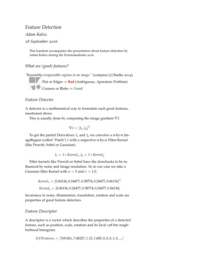
Feature Detection Adam Kalisz 18 September 2016 This handout accompanies the presentation about feature detection by Adam Kalisz during the Ferienakademie 2016 . What are (good) features? "Repeatably recognizable regions in an image." (compare [ 1 ] Radke 2014 ). Flat or Edges -> Bad (Ambiguous, Aperature Problem) Corners or Blobs -> Good Feature Detector A detector is a mathematical way to formulate such good features, mentioned above. This is usually done by computing the image gradient ∇ I . ∇ I = [ I x , I y ] T To get the partial Derivatives I x and I y we convolve a n-by-n Im- ageRegion (called "Patch") I with a respective n-by-n Filter-Kernel (like Prewitt, Sobel or Gaussian). I x = I ∗ Kernel x , I y = I ∗ Kernel y Filter kernels like Prewitt or Sobel have the drawbacks to be in- fluenced by noise and image resolution. So in our case we take a Gaussian filter Kernel with n = 5 and σ = 1.0: Kernel x = [ 0.06136, 0.24477, 0.38774, 0.24477, 0.06136 ] T Kernel y = [ 0.06136, 0.24477, 0.38774, 0.24477, 0.06136 ] Invariance to noise, illumination, translation, rotation and scale are properties of good feature detectors. Feature Descriptor A descriptor is a vector which describes the properties of a detected feature, such as position, scale, rotation and its local 128 bin neigh- borhood histogram. Si f tFeature 1 = [ 318.861, 7.48227, 1.12, 1.685, 0, 0, 0, 1, 0, .... ]

feature detection 2 Harris-Stephens Corner Detector Detector "The Harris corner detection algorithm [...] is one of the simplest corner indicators available" . (compare [ 3 ] Solem 2012 , p. 29 )      I 2  I x I x I y x M Image = ∇ I ∇ I T = � � I x I y =   I 2 I y I x I y y Using a Weight-Matrix we get a local averaging of the above Ma- trix over the neighboring pixels, often called the Harris Matrix : H = W ∗ M Image The Harris response is given by computing the eigenvalues of H or simpler by an indicator function, like this: det ( H ) H Response = det ( H ) − κ · trace ( H ) 2 ≈ trace ( H ) 2 Descriptor A possible way to create a descriptor for Harris features is through Normalized cross-correlation : ( I 1 ( � x ) − µ 1 ) · ( I 2 ( � x ) − µ 2 ) 1 n − 1 ∑ ncc ( I 1 , I 2 ) = σ 1 σ 2 � x The similarity of two images I 1 and I 2 is determined by the sum of all positions � x in image patches using the number of Pixels n in a patch, the mean intensities µ 1 and µ 2 as well as the standard devia- tions in each patch σ 1 and σ 2 . SIFT (Scale-Invariant-Feature-Transform) Detector The only possible scale-space kernel is the Gaussian: 1 2 πσ 2 e − ( x 2 + y 2 ) /2 σ 2 G ( x , y , σ ) = Hence we use it to define the scale-space of our image via convolu- tion: L ( x , y , σ ) = G ( x , y , σ ) ∗ I ( x , y ) We can use the scale-space extrema in the difference-of-Gaussian function D ( x , y , σ ) to efficiently detect stable keypoint locations:

feature detection 3 D ( x , y , σ ) = ( G ( x , y , k σ ) − G ( x , y , σ )) ∗ I ( x , y ) = L ( x , y , k σ ) − L ( x , y , σ ) The local extrema detection is accomplished by comparing a sam- ple point to its eight neighbors in the current image, as well as the nine neighbors in the scale above and below, like this: The sample point is considered a feature point only, if it differs by a certain threshold to all of these neighboring points. To improve the accuracy of the keypoint localization several filter- ing methods are being used (e.g. rejecting samples with low contrast or positioned along edges ). Additionally principal curvatures can be computed from a 2 x 2 Hessian matrix at the keypoint location utiliz- ing the efficient Harris-Stephens indicator function mentioned earlier. Descriptor In order to provide a robust way to compare features across multiple images, a vector containing unique attributes is assigned to each keypoint, such as magnitude and orientation of the gradient using pixel differences: � ( L ( x + 1, y ) − L ( x − 1, y )) 2 + ( L ( x , y + 1 ) − L ( x , y − 1 )) 2 m ( x , y ) = θ ( x , y ) = tan − 1 ( L ( x , y + 1 ) − L ( x , y − 1 ) L ( x + 1, y ) − L ( x − 1, y )) This can be visualized as follows:

feature detection 4 References [ 1 ] Rich Radke, 20 . 02 . 2014 , "CVFX Lecture 9 : Feature Detectors" , https://www.youtube.com/watch?v=9-F5-gUIAWE [ 2 ] Rich Radke, 24 . 02 . 2014 , "CVFX Lecture 10 : Feature descriptors" , https://www.youtube.com/watch?v=oFVexhcltzE [ 3 ] Jan Erik Solem, "Programming Computer Vision with Python" , 17 . 08 . 2012 , Print ISBN: 978 - 1 - 4493 - 1654 - 9 [ 4 ] Dr. Mubarak Shah, 19 . 09 . 2012 , "Lecture 04 - Interest Point Detec- tion" , https://www.youtube.com/watch?v=_qgKQGsuKeQ [ 5 ] Dr. Mubarak Shah, 19 . 09 . 2012 , "Lecture 05 - Scale-invariant Feature Transform (SIFT)" , https://www.youtube.com/watch?v=NPcMS49V5hg [ 6 ] David G. Lowe, 05 . 01 . 2004 , "Distinctive Image Features from Scale- Invariant Keypoints" , https://www.cs.ubc.ca/~lowe/papers/ijcv04. pdf [ 7 ] OpenCV, 28 . 08 . 2016 , "OpenCV: Introduction to SIFT (Scale-Invariant Feature Transform):" , http://docs.opencv.org/3.1.0/da/df5/tutorial_ py_sift_intro.html#gsc.tab=0