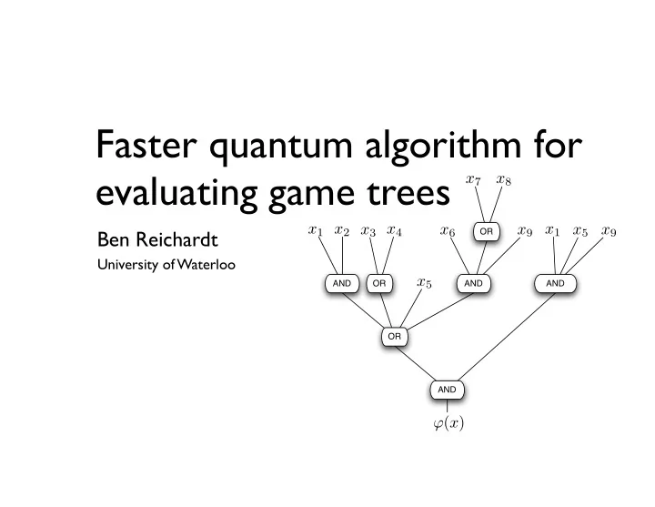
Faster quantum algorithm for evaluating game trees x 7 x 8 x 1 x 2 x - - PowerPoint PPT Presentation

Faster quantum algorithm for evaluating game trees

Ben Reichardt

x9 x5 x6

x9 x8 x7 x5 x4 x2 x3

AND OR AND AND AND OR OR

ϕ(x) x1 x1

University of Waterloo

x9 x5 x6

x9 x8 x7 x5 x4 x2 x3

AND OR AND AND AND OR OR

ϕ(x) x1 x1

x9 x5 x6

x9 x8 x7 x5 x4 x2 x3

AND OR AND AND AND OR OR

ϕ(x) x1 x1

Motivations:

• Two-player games (Chess, Go, …)
• Nodes ↔ game histories
• White wins iff ∃ move s.t. ∀ responses, ∃

move s.t. …

• Decision version of min-max tree

evaluation

• inputs are real numbers
• want to decide if minimax is ≥10 or not
• Model for studying effects of

composition on complexity

For balanced, binary formulas α-β pruning is optimal ⇒ Randomized complexity N0.754

x1 x2 x3 x4 x5 x7 x6 x8 ϕ(x)

[Snir ‘85, Saks & Wigderson ’86, Santha ’95]

Deterministic decision-tree complexity = N

Any deterministic algorithm for evaluating a read-once AND-OR formula must examine every leaf

N0.51 ≤ Randomized complexity ≤ N

[Heiman, Wigderson ’91] (see also K. Amano, Session 12B Tuesday)

Deterministic decision-tree complexity = N N0.51 ≤ Randomized complexity ≤ N Quantum query complexity = √N

(very special case of the next talk)

This talk: What is the time complexity for quantum algorithms?

U0

q u e r y x

U1

q u e r y x …

UT

f(x)

w/ prob. ≥2/3

|1 + |2 → (−1)x1|1 + (−1)x2|2 |x ∈ {0, 1}n| |j (−1)xj|j

OR AND OR AND AND AND AND

x1 x2 x3 x4 x5 x7 x6 x8 ϕ(x)

Farhi, Goldstone, Gutmann ’07 algorithm

• Theorem ([FGG ’07]): A balanced binary AND-OR formula can be evaluated

in time N½+o(1).

• Theorem ([FGG ’07]): A balanced binary AND-OR formula can be evaluated

in time N½+o(1).

• Convert formula to a tree, and attach a line to the root
• Add edges above leaf nodes evaluating to one

=0 =1

Farhi, Goldstone, Gutmann ’07 algorithm

OR AND OR AND AND AND AND

x1 x2 x3 x4 x5 x7 x6 x8 ϕ(x)

Farhi, Goldstone, Gutmann ’07 algorithm

• Theorem ([FGG ’07]): A balanced binary AND-OR formula can be evaluated

in time N½+o(1).

• Convert formula to a tree, and attach a line to the root
• Add edges above leaf nodes evaluating to one

x11 = 0 x11 = 1 =0 =1 ϕ(x) = 0 ϕ(x) = 1

|ψt = eiAGt|ψ0

ϕ(x) = 0 ϕ(x) = 1

|ψt = eiAGt|ψ0

Wave transmits! Wave reflects!

ϕ(x) = 0 ϕ(x) = 1

ϕ(x) = 0

What’s going on?

                          

Observe: State inside tree converges to

energy-zero eigenstate of the graph

ϕ(x) = 0

What’s going on?

=0 =1                           

Observe: State inside tree converges to

energy-zero eigenstate of the graph (supported on vertices that witness the formula’s value)

Energy-zero eigenvectors for AND & OR gadgets

• ⇔

OR: AND: +1 +1

• 1
• 1
• 1
• 1

Together in a formula: +1

• 1
• 1

+1 +1 Input adds constraints via dangling edges:

G

Balanced AND-OR formula evaluation in O(√n) time

Squared norm = +1

• 1
• 1

+1 +1 +1 +1 +1 +1 1 + 2 + 2 + 4 + 4 + 8 + 8 + · · · + 2

1 2 log2 n = O(√n)

· · · 1 2 2

Effective spectral gap lemma If M u ≠ 0, then M u ⊥ Kernel(M✝)

• by the SVD M =
• ρ

ρ |vρ uρ|

• projection of M u onto the

span of the left singular vectors

• f M with singular values ≤λ

≤ λ u

• since
• ΠM

u2 =

• ρ≤λ

ρ2|uρ|u|2

Squared norm = O(√n) 1 2 2 n¼

• 1
• 1

+1 +1 +1 +1 +1 +1 · · · 1/n¼ 1 / n¼

Case φ(x)=1

Constant overlap on root vertex

Case φ(x)=1

Eigenvalue-zero eigenvector with constant

• verlap on root vertex

Case φ(x)=0

• projection of M u onto the

span of the left singular vectors

• f M with singular values ≤λ

≤ λ u

• n
• 1
• 1

+1 +1 +1 +1 +1 +1 · · · 1/n 1/n

• · · ·

1/n¼ 1 / n¼ n¼

• n¼

n¼ n¼

u

• 1

M u

• root

√n

Root vertex has Ω(1/√n) effective spectral gap

Case φ(x)=1

Eigenvalue-zero eigenvector with constant

• verlap on root vertex

Case φ(x)=0

n

• 1
• 1

+1 +1 +1 +1 +1 +1 · · · 1/n 1/n

• Root vertex has

Ω(1/√n) effective spectral gap

· · · 1/n 1/n n

• n

n n

u

• 1

M u

• Quantum algorithm:

Run a quantum walk on the graph, for √n steps from the root.

• φ(x)=1 ⇒ walk is stationary
• φ(x)=0 ⇒ walk mixes

Evaluating unbalanced formulas

[Ambainis, Childs, Reichardt, Špalek, Zhang ’10]

Proper edge weights on an unbalanced formula give √(n·depth) queries depth n, spectral gap 1/n

“Rebalancing” Theorem:

For any AND-OR formula with n leaves, there is an equivalent formula with

n e√log n leaves, and depth e√log n

[Bshouty, Cleve, Eberly ’91, Bonet, Buss ’94]

O(√n e√log n) query algorithm

⇒

Today: O(√n log n)

Tensor-product composition

OR: AND:

Direct-sum composition

∨ ∧ ∨

Tensor-product composition Direct-sum composition

Tensor-product composition

∨ ∧

Properties

• Depth from root stays ≤2

— 1/√n spectral gap

• Graph stays sparse—

provided composition is along the maximally unbalanced formula

• Middle vertices Maximal

false inputs ↔ 010 100 0010 1100 01010 10010 00100

Final algorithm ∧ ∨ ∧ ∧

sort subformulas by size

• ⇔
• With direct-sum composition, large depth implies small spectral gap
• Tensor-product composition gives √n-query algorithm (optimal), but graph is

dense and norm too large for efficient implementation of quantum walk

• Hybrid approach:
• Decompose the formula into paths,

longer in less balanced areas

• Along each path, tensor-product
• Between paths, direct-sum
• Tradeoff gives 1/(√n log n) spectral gap,

while maintaining sparsity and small norm ⇒ Quantum walk has efficient implementation (poly-log n after preprocessing) ACRŠZ ’10 √n e√log n today √n log n